L. David Roper
http://roperld.com/personal/RoperLDavid.htm
29 November 2007
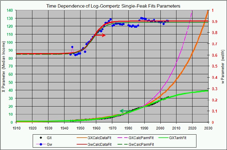
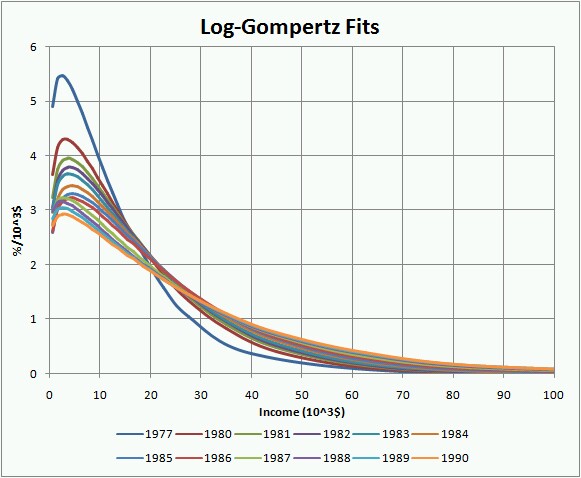
(This analysis was originally done in 1978 and included data from 1910 to 1977. Appendix IV extends the analysis to 2005.)
There is no more important subject in the economic history of a society than the history of the distribution of income. A knowledge of such history would enable a society to perceive its evolution and, perhaps, plan for gradual changes into more desirable directions in the future.
Ascertaining the history of the distribution of income is a task fraught with difficulty and uncertainty. Besides the problem of lack of data, there is also the problem of the meaning of the extant “data”. Even if the data were abundant and all investigators could agree on their meaning, then there is the problem of deciding how to summarize the data with a few parameters that characterize the income distribution as a function of time. I shall have to confront all of these problems in this paper.
In Section II the extant data are discussed; basically we accept the gross income data from 1944 to the present (1977), as collected by the U.S. Treasury Department, as valid data. In Section III we present a mathematical equation for the income distribution (the log-Verhulst function ); the parameters in this equation then serve to summarize the history of income distribution in the United States after the equation is fitted to the data by varying the parameters. One of the parameters is the median income; equations exist that relate it and the remaining parameters to, perhaps, more meaningful parameters such as modal income and average income. Until recent years more than one log-Verhulst function is required to fit the data; i.e., the data show structure that can be represented as a sum of several log-Verhulst peaks. Recently the data have been evolving toward a single log-Verhulst function.
Plots of the summarizing parameters versus time enable one to ascertain simple time behavior for them. I present simple mathematical expressions for this time dependence with included parameter values obtained by fitting the summarizing parameters as functions of time. These equations then enable one to project into the future. Current events make it obvious that the United States is entering an entirely new economic era. It will be interesting to see how well our projection agrees with the income distribution data for the next decade.
Some conclusions reached in this study are:
One would, of course, like to have a reliable set of income distribution data spanning the entire history of the United States. The existing situation is far from the ideal.
Probably the best summary of the U.S. income data situation is given in Historical Statistics of the U.S.: Colonial Times to 1970 (Ref. 1). (I shall refer to this reference as “ Historical Statistics”.) It references the isolated attempts to arrive at U.S. income distributions by Spahr (Ref.2) for 1896, King (Ref. 3) for 1910, Macauley (Ref. 4) for 1918, and Leven (Ref. 5) for 1929. I also use some 1936 data. I shall use these “data” to some small degree, but we really desire a more continuous set of data arrived at by more consistent and reliable means.
Historical Statistics states (Ref. 1) “Distribution of Federal individual income tax returns by income bracket are available annually since 1913. Before World War II the minimum filing requirements were relatively high so that the tabulations covered only a small fraction of the population. Successive lowering of the filing limit coupled with the rise in incomes after the depression of the 1930's led to a very marked expansion in coverage so that very few groups of the population are excluded in the postwar tabulations.”
Accordingly, we choose as our basic data set the U.S. gross income distribution from 1944 to the present, as reported in Statistics of Income (Ref. 6), a U.S. Treasury Department annual publication. In doing so we fully realize the limitations of that data; for example, the possibility of gross dishonesty in citizens reporting their income. Nevertheless, these data appear to be the most reliable data available. Of course, the conclusions that emerge from our study are no more reliable than are the data on which they are based. I would welcome a more reliable data base on which to base a future analysis.
I have tried to find the latest version of each year's distribution in Statistics of Income. I often choose a less complete revised distribution rather than the more complete distribution reported earlier, partly because we are not interested in "ultrafine" structure in the distributions.
Our set of distribution data are given in Appendix I in terms of percent of population per $1000 income (U.S. gross income distribution).
It should be pointed out that the income values are in absolute dollars, uncorrected for inflation.
Many researchers have, through the last several decades, attempted to fit income distributions with mathematical functions. I do not give a complete history of those attempts here. Instead we refer the reader to references 7 and 8.
Most of the previous work has concerned itself with fitting functions to the high-income tails of income distributions with, of course, the Pareto distribution (Ref. 9) being the favorite fitting function. Because we feel that this “fascination with the rich” helps little toward understanding the income situations of the majority of the citizens, we aim our study toward the entire income distribution, or at least the part of the distribution centered around the peak. (However, see Appendix V.)
Other investigators have studied the entire income distribution function and have attempted to fit functions to them (Ref. 9). However, most of those studies have not approached the details that are included in the study reported here.
As we shall show later, the log-Verhulst distribution function discussed in Appendix II fits the data better than does the lognormal distribution function, which is also discussed in Appendix II. Actually, in our best fits we use a sum of log-Verhulst functions in order to account for some of the fine structure in the data. The log-Verhulst distribution function is
![]() , where
, where ![]() (Eq. 1)
(Eq. 1)
(See Appendix II.)
The explicit dependence on x is
 . (Eq. 2)
The equation must be multiplied by 100 when fitting the income distribution data.
I fitted this function (or a sum of such functions) to the data by varying the parameters X, w, and n. When more than one function is used, we fitted
![]() (Eq. 3)
(Eq. 3)
to the data by varying the 4N-1 parameters
![]()
One interesting result of this study is that, when the data are fitted by only one log-Verhulst function, the best fit usually corresponds to n=0, which is a special limiting case of the log-Verhulst function called the log-Gompertz function. (See Appendix II.):
![]() (Eq. 4)
(Eq. 4)
or
The equation must be multiplied by 100 when fitting the income distribution data.
This function has the maximum “negative” skewness allowed by the log-Verhulst function. The fact that it fits the data best perhaps indicates the need for the selection or invention of another function with a greater negative skewness for fits to income distribution data. I do not consider such a possibility in this work.
There is good theoretical reasoning behind using logarithmic distributions for income distributions (Ref. 9), which we shall not discuss here. And certainly the distribution inside the logarithm should have the option of being non-symmetrical, which the normal distribution does not. Thus, it appears reasonable that the log-Verhulst distribution is a natural function for income distribution.
Fitting the data is a tedious process, requiring almost as much “art” as mathematics. I use the Microsoft Excel Solver procedure for doing the fits.
The fits to the data will be shown for all of the data and then the time dependence for the fit parameters will be discussed. The high-income tail will not be shown because our main interest is in the part of the distribution that is centered around the peak; that is, our interest is in the majority rather than in the rich.
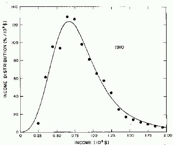
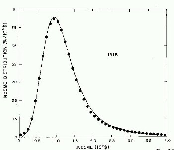
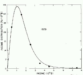
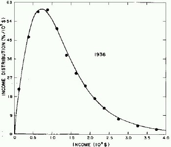
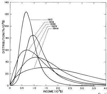
For the very crude data for 1910, 1918, 1929, and 1936 only one log-Verhulst distribution function is used for the fits. (In these cases the log-Gompertz function does not provide the best fits.) These fits are shown in Fig. 1.
Figure 1. Fits to the estimated income distributions for years prior to 1944 using a single log-Verhulst distribution function.
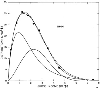
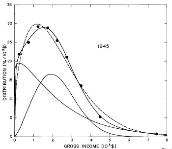
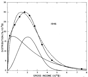
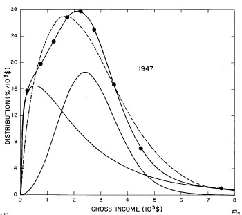
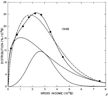
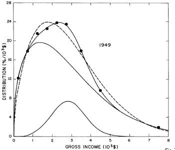
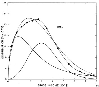
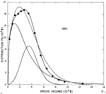
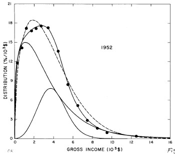
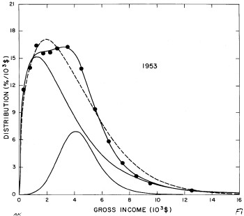
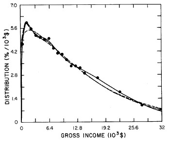
For the U.S. Treasury Department gross-income distribution data from 1944 to 1953 we did single-peak and double-peak fits, as shown in Figure 2. The single-peak fit is with the log-Gompertz function and the double-peak fit is with a sum of two log-Verhulst functions. Obviously, the double-peak fit is a significantly better fit to the data than is the single-peak fit; there is some time-dependent fine structure in the data which we shall discuss later. The relative ![]() values (
values ( ![]() =goodness of fit parameter; a lower
=goodness of fit parameter; a lower ![]() is a better fit) and the values of the fit parameters are given in Appendix III.
is a better fit) and the values of the fit parameters are given in Appendix III.
Figure 2. Fits to the U.S. Treasury Department gross-income distribution data from 1944 to 1953 using the log-Gompertz function for the single-peak fit (dashed curve) and a sum of two log-Verhulst functions for the double-peak fit. The two lower solid curves are the log-Verhulst functions and the upper solid curve is the sum of the two.
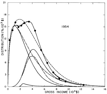
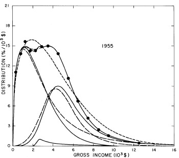
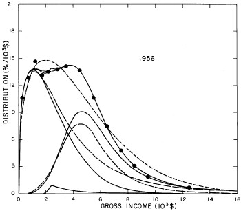
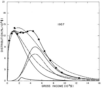
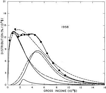
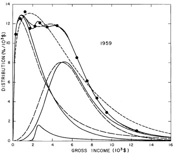
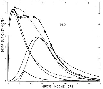
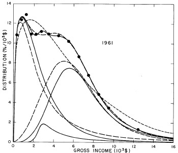
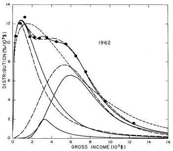
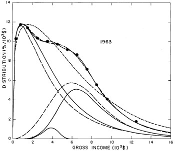
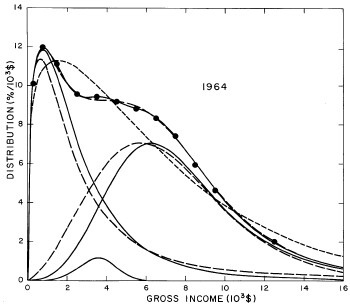
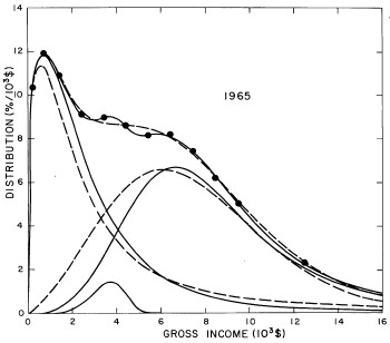
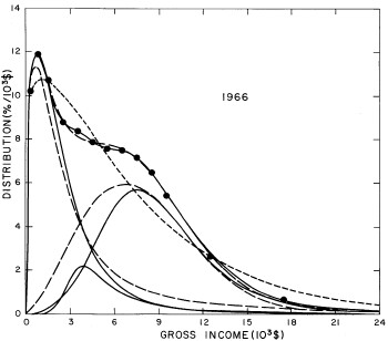
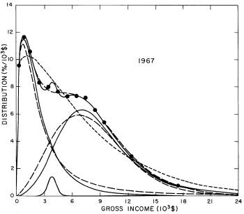
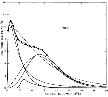
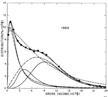
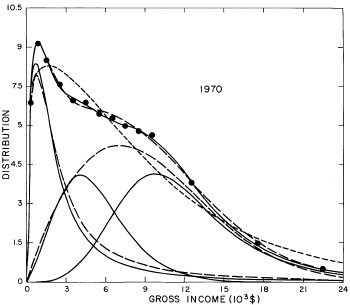
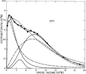
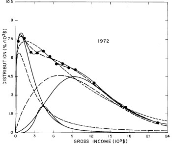
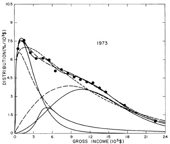
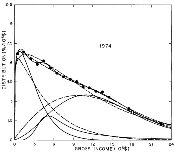
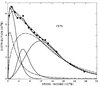
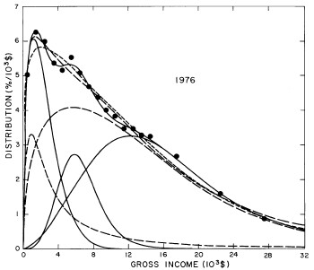
For the U.S. Treasury Department gross-income distribution data from 1954 to 1976 we find that a triple-peak fit to the data is significantly better than a double-peak or single-peak fit, although there still remains some structure unaccounted for by the triple-peak fit. Again, the single-peak fit is by means of the log-Gompertz function while the multiple-peak fits use the log-Verhulst function. The fits are shown in Fig. 3. The relative ![]() values and the values of the fit parameters are given in Appendix III. There are, perhaps, some bogus “wiggles” in some of our triple-peak fits (e.g., 1967); nevertheless, we feel that the triple-peak fit does represent quite well the behavior of the gross-income distribution. The time dependence of the fits’ parameters will be discussed later.
values and the values of the fit parameters are given in Appendix III. There are, perhaps, some bogus “wiggles” in some of our triple-peak fits (e.g., 1967); nevertheless, we feel that the triple-peak fit does represent quite well the behavior of the gross-income distribution. The time dependence of the fits’ parameters will be discussed later.
Figure 3. Fits to the U.S. Treasury Department gross-income distribution data for 1954-1976 using the log-Gompertz function for the single-peak fit (dotted curve) and a sum of log-Verhulst functions for the double-peak and triple-peak fits. The two lower dashed curves are the two log-Verhulst functions for the double-peak fit and the upper dashed curve is the sum of the two. The three lower solid curves are the three log-Verhulst functions for the triple-peak fit and the upper solid curve is the sum of the three.
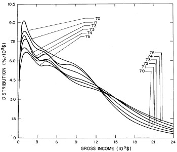
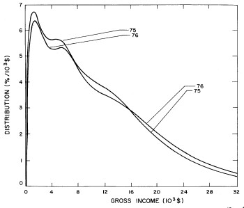
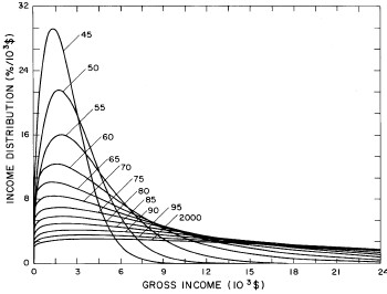
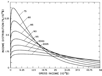
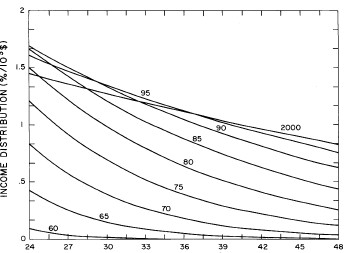
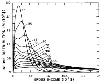
A more comprehensive view of the single-peak fits can be obtained by plotting several years together, as is done in Fig. 4.
Figure 4. Comparison of the single-peak fits for different years. Note that the border years for each graph are included on the next graph up or down.
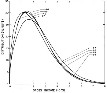
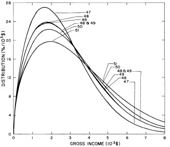
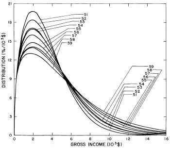
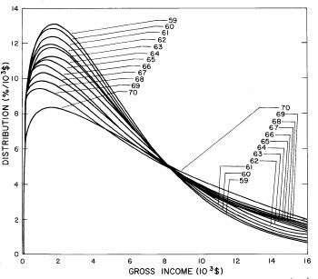
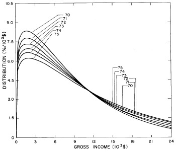
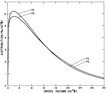
Probably the most noticeable feature is that, from 1944 to 1976 the peak of the distribution hovers between $1000 and $2000, even though the tail of the distribution steadily moves to higher incomes. This phenomenon will be discussed later.
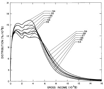
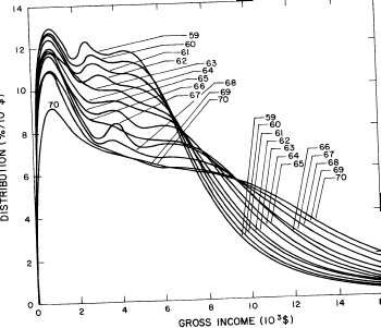
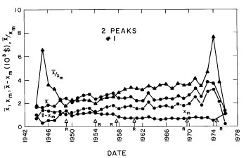
Similarly, the double-peak fits are plotted together in Fig. 5 and the triple-peak fits are plotted together in Fig. 6. One can easily see that the position of the lowest-income peak of the triple-peak fit is rather stable with time, which fact we shall discuss in greater detail later.
Figure. 5. Comparison of the double-peak fits for different years. Note that the border years for each graph are included on the next graph up and down.
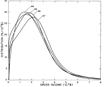
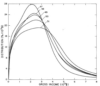
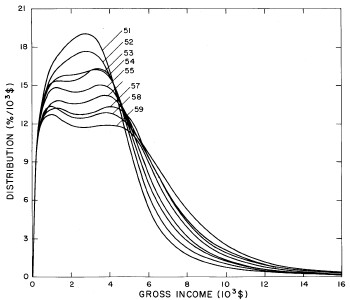
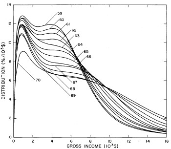
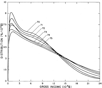
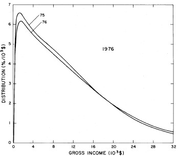
Figure 6. Comparison of the triple-peak fits for different years. Note that the border years for each graph are included on the next graph up and down.
Finally, to show that the log-Verhulst function fits the data better than the lognormal function, we compare the two fits for arbitrary years in Table 1.
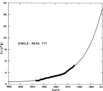
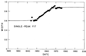
The single-peak fits given here are probably the best single-peak fits to the entire set of U.S. Treasury Department gross-income data that have ever been attained. Although the single-peak fits do not allow for some of the important structure in the data, for many purposes they may be sufficient. Therefore, we now discuss the single-peak fits in greater detail.
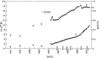
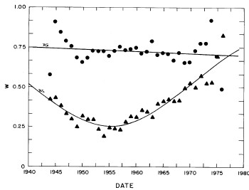
There are only two variable parameters in the log-Gompertz function, X (median income) and w (width). The values of these parameters for our fits are given in Appendix III and are shown in Fig. 7. (The years 1910, 1918, 1929, and 1936 are actually log-Verhulst fits, which include another parameter n, the asymmetry parameter.)
Figure 7. The parameters X (median income)(labeled x in the graph) and w (width) for the single-peak log-Gompertz fit to the 1944-1976 U.S. Treasury Department gross-income distribution data and for the log-Verhulst fit to the estimated 1910, 1918, 1929 and 1936 income data. The arrows on the date axis are the recessions as listed by Thurow (Ref 10.
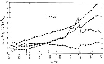
The modal income (X m, the income value at which the distribution has its maximum) is given by Eq. (18) in Appendix II. The values of the modal incomes for these fits are given in Appendix III and are shown in Fig. 8.
Figure 8. The parameter X (median income) (labeled ![]() in the graph) (upper solid line) and the calculated value of Xm (modal income) (lower solid line) for the single-peak log-Gompertz fit to the 1944-1976 U.S. Treasury Department gross income distribution data. Also shown as dashed lines are X-Xm and X/Xm. The arrows on the date axis are the recessions as listed by Thurow (Ref 10).
in the graph) (upper solid line) and the calculated value of Xm (modal income) (lower solid line) for the single-peak log-Gompertz fit to the 1944-1976 U.S. Treasury Department gross income distribution data. Also shown as dashed lines are X-Xm and X/Xm. The arrows on the date axis are the recessions as listed by Thurow (Ref 10).
If we exclude the crude data for dates earlier than 1944, the median income (X) values appear to rise approximately exponentially and the width (w) appears to change from one plateau to another. In fact, a fit of the function
to the X values and the function
to the w values yields the fits shown in Fig. 9 for the seven parameters ![]() given in Table 2.
given in Table 2.
Figure 9. The fit of Eq. (6) to the X values (labeled ![]() in the graph) and Eq. (7) to the w values determined by the single-peak log-Gompertz fits to the U.S. Treasury Department gross-income data for 1944-1976
in the graph) and Eq. (7) to the w values determined by the single-peak log-Gompertz fits to the U.S. Treasury Department gross-income data for 1944-1976
These curves can now be used, with some modest degree of confidence, to project U.S. gross-income distributions in the future or to calculate the distributions for years between 1944 and 1976.
Actually one should substitute (Eq. 6) and (Eq. 7) into (Eq. 5) and fit all of the 1944-1976 data (675 data) simultaneously by varying the seven parameters ![]() . This we have done and the resulting values of the seven parameters are given in Table 2.
. This we have done and the resulting values of the seven parameters are given in Table 2.
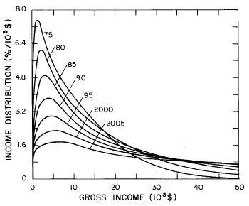
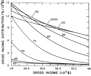
This simultaneous fit to all of the data is shown in Fig. 10. Sets of curves without the data and projections to the year 2005 are shown in Fig. 11.
Figure 10. Simultaneous single-peak log-Gompertz fit to all of the 1944-1976 U.S. Treasury Department gross-income distribution data using (Eq. 5), (Eq. 6) and (Eq. 7)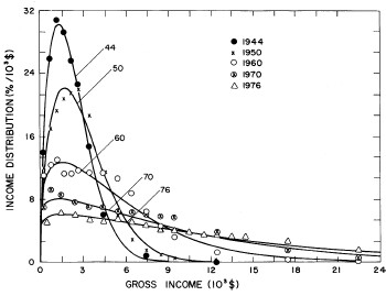
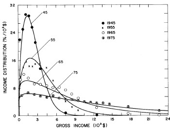
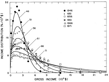
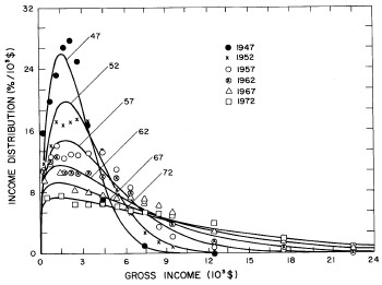
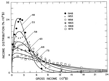
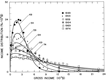
Figure 11. Curves for the fit shown in Fig. 10. for five-year intervals. Note in the last set of curves the income axis begins at 24x103$ rather than zero.
It may be that we are unjustified in assuming that w is at a plateau and will remain there to the year 2000 (see Fig. 7). However, w has been approximately at a plateau for the last decade and the mathematics of Eq. (5) does not permit it go much higher (maximum is 1 and it now hovers at about 0.88). If it is to change appreciably in the future it must drop, which would mean that the income distribution would constrict; i.e., the spread in the distribution would narrow, which is contrary to essentially all of the past history of the U.S. income distribution.
Also, our crude representation of X by an exponential function could be improved by using other functions. E.g., perhaps a hyperbola would be better (see Fig. 7 and Fig. 9) or a series of joined straight lines.
However, note that our single-peak log-Gompertz fits are quite good for the most recent data (see Fig. 3 and Fig. 10). So one might believe that our extrapolations to the year 2000 are reasonable.
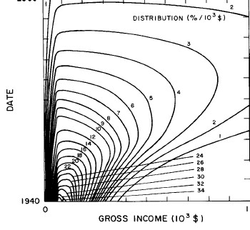
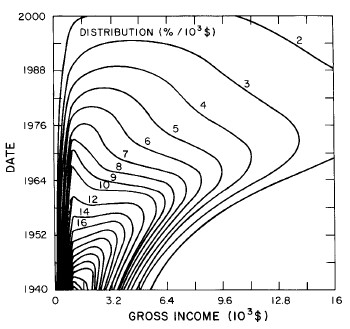
Another way to get a “feel” for the behavior with time and income for the U.S. gross-income distribution is to do a three-dimensional plot of our single-peak log-Gompertz fit. This is shown in Fig. 12. Also, in Fig. 13 are shown contour plots. These curves make very obvious the rapid changes in income distribution that occurred after World War II and the recent slowing of changes.
Figure 12. Three-dimensional plots of the curves for the fit shown in Fig. 10. The first three graphs are views from different “directions”. The interval markers are 2 years for the date axis and 103$ for the income axis. The last graph is an attempt to show how the curves behave for x<2x10³$; here the income interval markers are 125$.
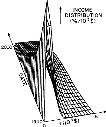
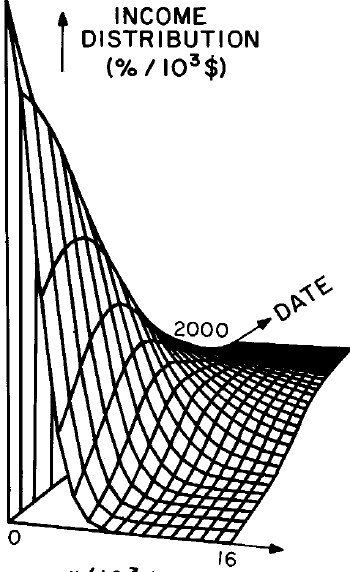
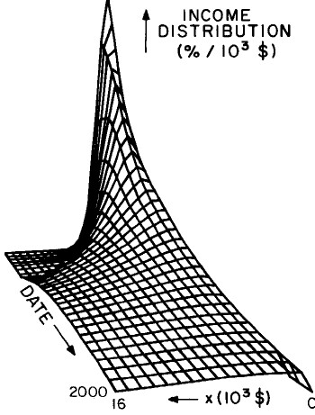
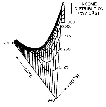
Figure 13. Contour plot of the curves for the fit shown in Fig. 10.
In Section VII, we shall discuss some of the salient features of the fits reported in this section.
The double-peak fits to the 1944-1976 U.S. Treasury Department gross income data are considerably better fits to the data than are the single-peak fits. In fact, they are quite decent fits. Those who are interested in greater accuracy than our single-peak fits give, should be able to obtain all of the accuracy that is usually justified in these matters by using our double-peak fit.
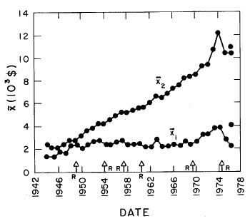
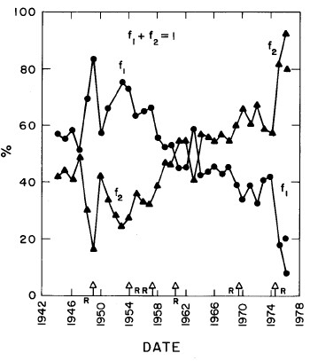
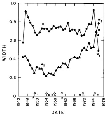
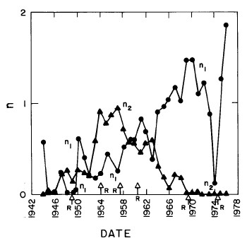
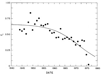
In most cases both of the peaks are the log-Verhulst functions. (Where the log-Gompertz function is used is indicated by a zero value for the asymmetry parameter n.) There are seven parameters for each year in the fits: the two median incomes (X1 and X2), the two "widths" (w1 and w2), the two asymmetry parameters (n1 and n2), and the fraction of the total for which the first peak accounts ( f1; f2 = f1-1) The values of these parameters for our fits are given in Appendix III and are shown in Fig. 14.
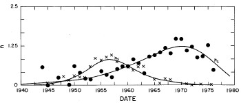
Figure 14. The parameters, X (median income) (labeled ![]() in the graph) , f (fraction due to peak #1), w (width) and n (asymmetry parameter) for the double-peak log-Verhulst fit to the 1944-1976 U.S. Treasury Department gross-income distribution data. The arrows on the date axis are the recessions as listed by Thurow (Ref. 10).
in the graph) , f (fraction due to peak #1), w (width) and n (asymmetry parameter) for the double-peak log-Verhulst fit to the 1944-1976 U.S. Treasury Department gross-income distribution data. The arrows on the date axis are the recessions as listed by Thurow (Ref. 10).
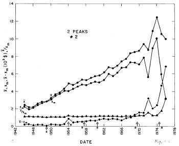
The modal incomes for the two peaks (xm1 and xm2) are given by Eq. (17) in Appendix II. The values of the modal incomes for these fits are given in Appendix III and are shown in Fig. 15.
Figure 15. The parameter X (median income) (upper solid line) and the calculated value of Xm (modal income) (lower solid line) for the double-peak log-Verhulst fit to the 1944-1976 U.S. Treasury Department gross-income distribution data. Also shown as dashed lines are X-Xm and X/Xm. The arrows on the date axis are the recessions as listed by Thurow (Ref. 10).
I fitted the following functions to the ![]() values given in Appendix III and obtained the fits shown in Fig. 16.
values given in Appendix III and obtained the fits shown in Fig. 16.
and
The parameters’ values for the fits are given in Table 3.
Figure 16. The fits of (Eq. 8) to the X values, of Eq. (9) to the f1 values, of (Eq. 10) and (Eq. 11) to the w values, and of (Eq. 12) and (Eq. 13) to the n values determined by double-peak log-Verhulst fits to the U.S. Treasury Department gross-income distribution data for 1944-1976. Note that we chose a different set of fits for recent years than the almost comparable sets of Fig, 14. I did this for continuity; it was possibly bad judgment.
Actually one should substitute (Eq. 8) through (Eq. 13) into (Eq. 3) and fit all of the 1944-1976 data (675 data) simultaneously by varying the twenty-two parameters. I have done this and the resulting values of the parameters are given in Tables 3.
This simultaneous fit to all of the data is shown in Fig. 17. Sets of curves without the data and projections to the year 2005 are shown in Fig.18.
Figure 17. Simultaneous double-peak log-Verhulst fit to all of the 1944-1976 U.S. Treasury Department gross-income distribution data using (Eq. 5) and (Eq. 8) through (Eq. 13).
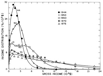
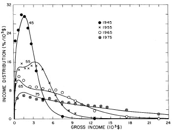
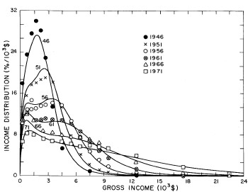
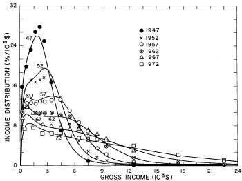
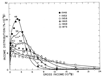
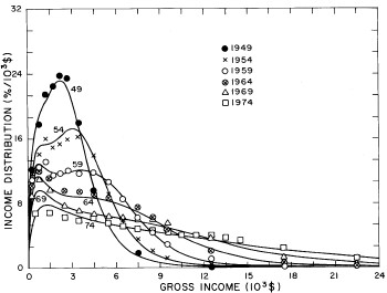
Figure 18. Curves for the fit shown in Fig. 17 in five-year intervals. Note that in the last graph the income axis begins at 23x103$ rather than zero.
Another way to get an overall view of the behavior of the income distribution with time and income is to plot in three dimensions our two-peak log-Verhulst fits. This is shown in Fig. 19. Also, in Fig. 20 are shown contour plots.
Figure 19. Three-dimensional plots of the curves for the fit shown in Fig. 17. The four graphs are views from different “directions”. The interval markers are 2 years for the date axis and 103$ for the income axis.
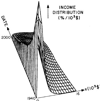
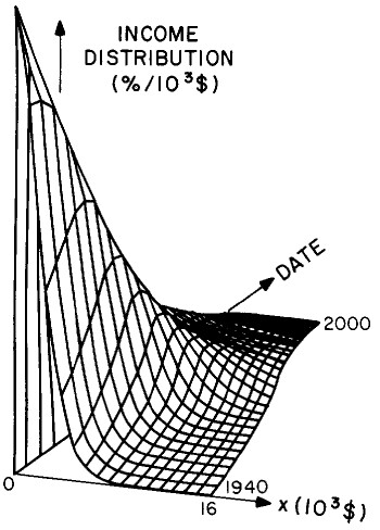
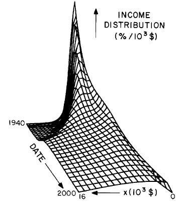
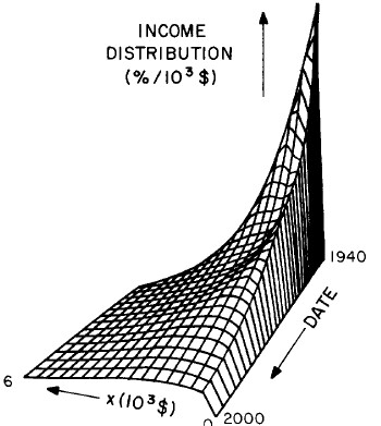
Figure 20. Contour plot of the curves for the fit shown in Fig. 17.
In the next section we shall discuss some of the salient features of the fits reported in this section.
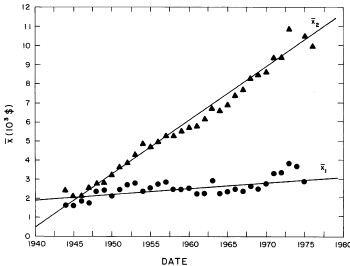
The 1944-1976 Treasury Department gross income data are well represented by a sum of two Verhulst functions, one for low income and one for high income. The high-income function has been steadily growing in size as the low-income function decreased in size. However, those ~20% of the population that are still in the low-income group have only about $1000 more median income than that group had in the 1940's when it contained about 60% of the population; whereas the higher-income group's median income rose from ~$2000 to ~$11,000 in that time interval.
For recent years, the single Verhulst function fits the data almost as well as two functions. Therefore, we feel that our single-function fit is a good extrapolator for the future. In fact, the 1977 data, which were not available when we did the original fits, are quite well represented by such an extrapolation, which is shown in Fig. 21. Fig. 22 shows the fits to the 1977 data.
Figure 21. Comparison of the 1977 gross income distribution data, single-peak log-Gompertz projection (solid curve) and the double-peak log-Verhulst projection (dashed curve). The poorness of the latter projection is probably due to our poor judgment in choosing one set of fits to recent data (Fig. 16) over another almost comparable set (Fig. 14). I felt that it was not worth redoing the two-peak projector, because the single-peak one is probably sufficient for projection purposes.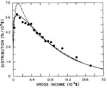
Figure 22. Fits to the U.S. Treasury Department gross-income distribution data for 1977 using the log-Gompertz function for the single-peak fit (dotted curve) and a sum of log-Verhulst functions for the double-peak fit (dashed curve) and triple-peak fit (solid curve).
A good measure of equity in income distribution is the ratio of the median income to the modal income (peak income). A ratio of 1 indicates that the distribution has as many people below the peak as above it. A ratio much greater than 1 indicates that some people are far richer than others. Figure 8 show that ratio for the single-function fit to the data. It has grown from about 1.5 in the 1940's to about 4.5 now. The fact that some people have greatly overtaken many others is also obvious by merely looking at the income distribution data. The income distribution is much more widely spread now than it was immediately after World War I. That wide spread is also indicated by the fact that the Verhulst function widths in both the single-peak and double-peak fits are now at about the maximum allowed values for the Verhulst function.
It will be interesting to observe in the coming years whether our single-peak fit will be a good predictor of U.S. income distribution. I include the complete equations here to allow ease of use by courageous forecasters:
where ![]() ,
,  .
.
Note that ![]() is the probability; it must be multiplied by 100 to get percentage.
is the probability; it must be multiplied by 100 to get percentage.
Some interesting questions that perhaps the future will answer are:
I close by noting that, with the detailed knowledge of its income distribution evolution provided by our work, the United States could design its tax laws to gradually change that evolution, if such seemed desirable.
The distribution is calculated as follows:
The factor 1000 converts the income range to units of $1000 and the 100 factor converts the fraction to %.
N=number of reporting units; first and fourth columns are income range in 103$.
|
1910 |
1918 |
1929 |
1936 |
|
N(10 6) |
27.945 |
37.369 |
|
48.5 |
39.458 |
0-0.1 |
0.36 |
1.681 |
0-0.25 |
31.901 |
21.532 |
0.1-0.2 |
V |
2.775 |
0.25-0.5 |
| |
46.500 |
0.2-0.3 |
9.66 |
5.596 |
0.5-0.75 |
| |
58.513 |
0.3-0.4 |
61.30 |
13.112 |
0.75-1 |
V |
59.567 |
0.4-0.5 |
95.37 |
25.743 |
1-1.25 |
41.480 |
50.596 |
0.5-0.6 |
93.76 |
41.478 |
1.25-1.5 |
| |
37.944 |
0.6-0.7 |
128.47 |
57.641 |
1.5-1.75 |
| |
29.297 |
0.7-0.8 |
126.14 |
71.396 |
1.75-2 |
V |
23.275 |
0.8-0.9 |
97.94 |
80.628 |
2-2.25 |
18.480 |
17.284 |
0.9-1.0 |
80.95 |
84.161 |
2.25-2.5 |
| |
12.712 |
1.0-1.1 |
65.34 |
82.261 |
2.5-3 |
V |
7.476 |
1.1-1.2 |
57.33 |
76.293 |
3-3.5 |
4.113 |
4.318 |
1.2-1.3 |
43.94 |
67.837 |
3.5-4 |
V |
2.545 |
1.3-1.4 |
25.4 |
59.033 |
4-4.5 |
1.485 |
1.450 |
1.4-1.5 |
17.0 |
49.025 |
4.5-5 |
V |
0.9027 |
1.5-1.6 |
13.8 |
40.488 |
5-7.5 |
0.3179 |
0.3855 |
1.6-1.7 |
11.0 |
33.022 |
7.5-10 |
V |
0.2186 |
1.7-1.8 |
8.70 |
26.760 |
10-15 |
0.04672 |
0.06371 |
1.8-1.9 |
6.76 |
21.708 |
15-20 |
| |
0.03443 |
1.8-2.0 |
5.08 |
17.763 |
20-25 |
V |
0.02019 |
2.0-2.1 |
3.58 |
14.713 |
25-30 |
0.006354 |
0.01297 |
2.1-2.2 |
V |
12.395 |
30-40 |
| |
0.004552 |
2.2-2.3 |
2.99 |
10.573 |
40-50 |
V |
0.002114 |
2.3-2.4 |
V |
9.101 |
50-100 |
0.001155 |
0.0006610 |
2.4-2.5 |
2.52 |
7.908 |
100-250 |
0.0001601 |
0.7002x10 -4 |
2.5-2.6 |
V |
6.923 |
250-500 |
0.2344x10 -4 |
0.9286x10 -5 |
2.6-2.7 |
2.06 |
6.093 |
500-1000 |
0.4012x10 -5 |
0.1276x10 -5 |
2.7-2.8 |
V |
5.392 |
|
|
|
2.8-2.9 |
1.68 |
4.787 |
|
|
|
2.9-3.0 |
V |
4.134 |
|
|
|
3.0-3.1 |
1.38 |
3.821 |
|
|
|
3.1-3.2 |
V |
3.431 |
|
|
|
3.2-3.3 |
1.13 |
3.093 |
|
|
|
3.3-3.4 |
V |
2.796 |
|
|
|
3.4-3.5 |
0.930 |
2.537 |
|
|
|
3.5-3.6 |
V |
2.312 |
|
|
|
3.6-3.7 |
0.769 |
2.115 |
|
|
|
3.7-3.8 |
V |
1.942 |
|
|
|
3.8-3.9 |
0.644 |
1.790 |
|
|
|
3.9-4.0 |
V |
1.656 |
|
|
|
4.0-4.4 |
0.528 |
1.152 |
|
|
|
4.4-4.8 |
0.438 |
| |
|
|
|
4.8-5.0 |
0.358 |
V |
|
|
|
5.0-5.2 |
V |
0.6281 |
|
|
|
5.2-5.6 |
0.286 |
| |
|
|
|
5.6-6.0 |
0.224 |
V |
|
|
|
6-7 |
0.165 |
0.3835 |
|
|
|
7-8 |
0.118 |
0.2540 |
|
|
|
8-9 |
0.0680 |
0.1780 |
|
|
|
9-10 |
V |
0.1294 |
|
|
|
10-11 |
0.0394 |
0.09749 |
|
|
|
11-12 |
V |
0.07576 |
|
|
|
12-13 |
0.277 |
0.06013 |
|
|
|
13-14 |
| |
0.04862 |
|
|
|
14-15 |
| |
0.04001 |
|
|
|
15-16 |
V |
0.02508 |
|
|
|
16-20 |
0.0179 |
V |
|
|
|
20-25 |
0.0072 |
0.01331 |
|
|
|
25-30 |
V |
0.008140 |
|
|
|
30-40 |
0.0043 |
0.004565 |
|
|
|
40-50 |
0.0025 |
0.002369 |
|
|
|
50-60 |
0.0008323 |
0.001397 |
|
|
|
60-70 |
| |
0.0009069 |
|
|
|
70-80 |
| |
0.0006318 |
|
|
|
80-90 |
| |
0.0004630 |
|
|
|
90-100 |
V |
0.0003508 |
|
|
|
100-150 |
0.0001125 |
1.870x10 -4 |
|
|
|
150-200 |
V |
7.766x10 -5 |
|
|
|
200-250 |
0.117x10 -5 |
4.13x10 -5 |
|
|
|
250-300 |
| |
0.246x10 -4 |
|
|
|
300-400 |
| |
0.133x10 -4 |
|
|
|
400-500 |
| |
0.664x10 -5 |
|
|
|
500-750 |
| |
0.284x10 -5 |
|
|
|
750-1000 |
V |
0.111x10 -5 |
|
|
|
1000-1500 |
3.5x10 -7 |
0.42x10 -6 |
|
|
|
1500-2000 |
V |
0.16x10 -6 |
|
|
|
2000-3000 |
4.9x10 -8 |
0.64x10 -7 |
|
|
|
3000-4000 |
| |
0.24x10 -7 |
|
|
|
4000-5000 |
V |
|
|
|
|
5000-10000 |
7.2x10 -9 |
|
|
|
|
10000-50000 |
4.5x10 -10 |
|
|
|
|
# |
50 |
73 |
|
12 |
27 |
|
1944 |
1945 |
1946 |
1947 |
1948 |
1949 |
1950 |
N(10 6) |
46.920 |
49.751 |
52.600 |
54.800 |
51.746 |
51.302 |
52.656 |
0.001-0.5 |
13.900 |
21.917 |
17.932 |
15.752 |
12.755 |
12.214 |
|
0.5-1 |
25.865 |
24.976 |
23.475 |
19.847 |
17.281 |
17.867 |
|
0.001-0.6 |
|
|
|
|
|
|
11.964 |
0.6-1 |
|
|
|
|
|
|
17.007 |
1-1.5 |
30.786 |
29.225 |
27.601 |
23.223 |
20.017 |
21.559 |
19.284 |
1.5-2 |
29.258 |
28.848 |
30.015 |
26.854 |
23.059 |
22.580 |
20.788 |
2-2.5 |
25.575 |
25.519 |
28.255 |
27.759 |
24.334 |
23.812 |
21.433 |
2.5-3 |
22.596 |
21.113 |
22.894 |
24.985 |
23.820 |
23.508 |
21.977 |
3-4 |
14.746 |
13.541 |
13.376 |
16.721 |
18.160 |
17.939 |
18.682 |
4-5 |
6.004 |
5.252 |
5.317 |
7.093 |
9.846 |
19.620 |
11.366 |
5-6 |
0.7818 |
0.7578 |
0.8867 |
1.036 |
1.803 |
1.886 |
5.745 |
6-7 |
| |
| |
| |
| |
| |
| |
2.894 |
7-8 |
| |
| |
| |
| |
| |
| |
1.514 |
8-9 |
| |
| |
| |
| |
| |
| |
0.8916 |
9-10 |
V |
V |
V |
V |
V |
V |
0.5682 |
10-11 |
0.1272 |
0.1420 |
0.1720 |
0.1777 |
0.2317 |
0.2267 |
0.2579 |
11-12 |
| |
| |
| |
| |
| |
| |
| |
12-13 |
| |
| |
| |
| |
| |
| |
| |
13-14 |
| |
| |
| |
| |
| |
| |
| |
14-15 |
V |
V |
V |
V |
V |
V |
V |
15-20 |
0.05520 |
0.06243 |
0.07319 |
0.07347 |
0.09137 |
0.08592 |
0.09723 |
20-25 |
0.02879 |
0.03346 |
0.03816 |
0.03737 |
0.04723 |
0.04538 |
0.05310 |
25-30 |
0.008568 |
0.009664 |
0.01104 |
0.01072 |
0.01431 |
0.01336 |
0.03177 |
30-50 |
V |
V |
V |
V |
V |
V |
0.01296 |
50-100 |
0.001234 |
0.001347 |
0.001487 |
0.001389 |
0.002038 |
0.001798 |
0.002381 |
100-150 |
0.0002077 |
0.0002223 |
0.0002423 |
0.0002319 |
0.0003718 |
0.0003130 |
0.0004391 |
150-200 |
|
|
|
|
|
|
0.0001500 |
200-500 |
|
|
|
|
|
|
2.569x10 -5 |
150-300 |
0.3667x10 -4 |
0.3847x10 -4 |
0.4232x10 -4 |
0.4157x10 -4 |
0.6629x10 -4 |
0.5874x10 -4 |
|
300-500 |
0.3360x10 -5 |
0.531x10 -5 |
0.620x10 -5 |
0.600x10 -5 |
0.920x10 -5 |
0.755x10 -5 |
|
500-1000 |
0.9420x10 -6 |
0.104x10 -5 |
0.123x10 -5 |
0.110x10 -5 |
0.148x10 -5 |
0.148x10 -5 |
2.37x10 -6 |
# |
18 |
18 |
18 |
18 |
18 |
18 |
23 |
|
1951 |
1952 |
1953 |
1954 |
1955 |
1956 |
1957 |
N(10 6) |
55.043 |
56.107 |
57.416 |
56.307 |
57.818 |
58.799 |
59.408 |
0.001-0.6 |
11.603 |
11.781 |
11.588 |
11.662 |
11.066 |
10.073 |
10.753 |
0.6-1 |
15.483 |
14.094 |
13.981 |
14.124 |
13.850 |
12.871 |
12.582 |
1-1.5 |
17.684 |
17.146 |
16.417 |
16.059 |
15.649 |
14.677 |
14.065 |
1.5-2 |
18.022 |
16.796 |
15.574 |
14.943 |
14.269 |
13.119 |
12.453 |
2-2.5 |
18.694 |
17.132 |
15.654 |
15.316 |
14.242 |
13.561 |
12.937 |
2.5-3 |
19.051 |
17.520 |
16.100 |
15.931 |
14.916 |
13.799 |
12.844 |
3-4 |
18.164 |
17.265 |
16.271 |
16.261 |
14.987 |
14.084 |
13.116 |
4-5 |
13.208 |
13.606 |
13.903 |
14.050 |
13.852 |
13.686 |
13.244 |
5-6 |
7.480 |
8.414 |
9.392 |
9.215 |
10.140 |
10.604 |
11.034 |
6-7 |
4.117 |
5.149 |
5.828 |
5.953 |
6.697 |
7.436 |
7.928 |
7-8 |
2.204 |
2.832 |
3.466 |
3.582 |
4.151 |
4.759 |
5.399 |
8-9 |
1.256 |
1.595 |
2.012 |
2.108 |
2.444 |
3.080 |
3.520 |
9-10 |
0.7569 |
0.9327 |
1.226 |
1.281 |
1.578 |
1.910 |
2.248 |
10-11 |
0.3023 |
0.3505 |
0.4040 |
0.4323 |
0.5251 |
0.6534 |
0.7454 |
11-12 |
| |
| |
| |
| |
| |
| |
| |
12-13 |
| |
| |
| |
| |
| |
| |
| |
13-14 |
| |
| |
| |
| |
| |
| |
| |
14-15 |
V |
V |
V |
V |
V |
V |
V |
15-20 |
0.1076 |
0.1156 |
0.1218 |
0.1310 |
0.1474 |
0.1694 |
0.1831 |
20-25 |
0.05625 |
0.04499 |
0.04611 |
0.05184 |
0.07275 |
0.07990 |
0.08447 |
25-30 |
0.03405 |
V |
V |
V |
0.04172 |
0.02357 |
0.02467 |
30-50 |
0.01361 |
0.01363 |
0.01316 |
0.01438 |
0.01649 |
V |
V |
50-100 |
0.002451 |
0.002331 |
0.002100 |
0.002500 |
0.002684 |
0.003033 |
0.003145 |
100-150 |
0.0004378 |
0.0002515 |
0.0002175 |
0.0004131 |
0.0004483 |
0.0004799 |
0.0004757 |
150-200 |
0.0001456 |
V |
V |
0.0001136 |
0.0001365 |
0.0001310 |
0.0001348 |
200-500 |
0.2365x10 -4 |
0.1901x10 -4 |
0.1567x10 -4 |
0.1921x10 -4 |
0.2319x10 -4 |
0.2293x10 -4 |
0.2243x10 -4 |
500-1000 |
0.190x10 -5 |
0.148x10 -5 |
0.130x10 -5 |
0.156x10 -5 |
0.217x10 -5 |
0.203x10 -5 |
0.197x10 -5 |
# |
23 |
21 |
21 |
22 |
23 |
22 |
22 |
|
1958 |
1959 |
1960 |
1961 |
1962 |
1963 |
1964 |
N(10 6) |
58.701 |
58.838 |
60.593 |
61.068 |
62.291 |
63.511 |
64.943 |
0.001-0.6 |
11.215 |
10.916 |
10.977 |
10.832 |
10.708 |
10.368 |
10.106 |
0.6-1 |
13.032 |
12.517 |
12.349 |
12.360 |
12.048 |
11.770 |
11.964 |
1-1.5 |
14.037 |
13.219 |
13.012 |
12.893 |
12.695 |
11.425 |
11.092 |
1.5-2 |
12.167 |
11.515 |
11.272 |
10.899 |
10.637 |
V |
V |
2-2.5 |
12.569 |
11.731 |
11.239 |
10.909 |
10.573 |
10.359 |
9.563 |
2.5-3 |
12.688 |
12.093 |
11.615 |
11.177 |
10.486 |
V |
V |
3-4 |
12.729 |
11.688 |
11.350 |
10.963 |
10.576 |
10.022 |
9.431 |
4-5 |
12.581 |
11.819 |
11.333 |
10.780 |
10.083 |
9.772 |
9.200 |
5-6 |
10.862 |
10.684 |
10.601 |
10.196 |
9.886 |
9.190 |
8.850 |
6-7 |
7.968 |
8.495 |
8.733 |
8.650 |
8.627 |
8.619 |
8.338 |
7-8 |
5.498 |
6.183 |
6.418 |
0.785 |
6.954 |
7.164 |
7.449 |
8-9 |
3.700 |
4.380 |
4.551 |
4.888 |
5.208 |
5.566 |
5.968 |
9-10 |
2.475 |
2.925 |
3.145 |
3.516 |
3.859 |
4.174 |
4.661 |
10-11 |
0.8477 |
1.073 |
1.203 |
1.350 |
1.586 |
1.784 |
2.035 |
11-12 |
| |
| |
| |
| |
| |
| |
| |
12-13 |
| |
| |
| |
| |
| |
| |
| |
13-14 |
| |
| |
| |
| |
| |
| |
| |
14-15 |
V |
V |
V |
V |
V |
V |
V |
15-20 |
0.2004 |
0.2364 |
0.2594 |
0.2913 |
0.3365 |
0.3898 |
0.4496 |
20-25 |
0.09019 |
0.1008 |
0.1069 |
0.1170 |
0.1303 |
0.1448 |
0.06221 |
25-30 |
0.02520 |
0.02825 |
0.02914 |
0.03253 |
0.03451 |
0.03121 |
|
30-50 |
V |
V |
V |
V |
V |
V |
V |
50-100 |
0.003125 |
0.003841 |
0.003344 |
0.003619 |
0.003904 |
0.004169 |
0.004902 |
100-150 |
0.0004797 |
0.0005862 |
0.0004693 |
0.0005499 |
0.0005067 |
0.0003593 |
0.0001345 |
150-200 |
0.0001317 |
0.0001503 |
0.0001456 |
0.0001788 |
0.0001622 |
V |
| |
200-500 |
0.227x10 -4 |
0.2679x10 -4 |
0.2667x10 -4 |
0.3331x10 -4 |
0.2765x10 -4 |
0.2882x10 -4 |
V |
500-1000 |
0.183x10 -5 |
0.241x10 -5 |
0.243x10 -5 |
0.323x10 -5 |
0.264x10 -5 |
0.257x10 -5 |
0.3305x10 -5 |
# |
22 |
22 |
22 |
22 |
22 |
19 |
17 |
|
1965 |
1966 |
1967 |
1968 |
1969 |
1970 |
1971 |
N(10 6) |
67.199 |
69.786 |
71.283 |
73.347 |
75.376 |
73.862 |
74.146 |
0.001-0.6 |
10.367 |
10.224 |
9.540 |
9.414 |
8.807 |
6.893 |
6.657 |
0.6-1 |
11.931 |
11.915 |
11.640 |
10.941 |
0.975 |
9.155 |
8.277 |
1-1.5 |
10.860 |
10.727 |
10.609 |
10.181 |
9.662 |
8.513 |
8.036 |
1.5-2 |
V |
V |
V |
V |
V |
V |
V |
2-2.5 |
9.121 |
8.787 |
8.284 |
8.039 |
7.811 |
7.594 |
7.242 |
2.5-3 |
V |
V |
V |
V |
V |
V |
V |
3-4 |
8.987 |
8.383 |
7.992 |
7.587 |
7.144 |
6.968 |
6,813 |
4-5 |
8.583 |
7.888 |
7.647 |
7.197 |
6.765 |
6.886 |
6.644 |
5-6 |
8.127 |
7.560 |
7.276 |
6.814 |
6.419 |
6.446 |
6.193 |
6-7 |
8.182 |
7.482 |
7.322 |
6.757 |
6.058 |
6.302 |
5.738 |
7-8 |
7.411 |
7.153 |
7.171 |
6.467 |
6.227 |
5.997 |
5.931 |
8-9 |
6.172 |
6.479 |
6.282 |
6.290 |
5.819 |
5.800 |
5.650 |
9-10 |
5.042 |
15.427 |
5.386 |
5.486 |
5.538 |
5.651 |
5.406 |
10-11 |
2.296 |
2.655 |
2.914 |
3.268 |
3.622 |
3.819 |
3.939 |
11-12 |
| |
| |
| |
| |
| |
| |
| |
12-13 |
| |
| |
| |
| |
| |
| |
| |
13-14 |
| |
| |
| |
| |
| |
| |
| |
14-15 |
V |
V |
V |
V |
V |
V |
V |
15-20 |
0.5244 |
0.6391 |
0.7749 |
0.9983 |
1.253 |
1.499 |
1.741 |
20-25 |
0.06915 |
0.07853 |
0.09156 |
0.3221 |
0.4079 |
0.5169 |
0.6414 |
25-30 |
| |
| |
| |
0.1419 |
0.1713 |
0.2080 |
0.2613 |
30-50 |
V |
V |
V |
0.4904 |
0.05356 |
0.06216 |
0.07268 |
50-100 |
0.005616 |
0.006259 |
0.007312 |
0.008230 |
0.008714 |
0.009504 |
0.01091 |
100-150 |
0.0001636 |
0.005866 |
0.0007204 |
0.0008590 |
0.0008438 |
0.0008458 |
0.0009826 |
150-200 |
| |
V |
V |
V |
V |
V |
V |
200-500 |
V |
0.4778x10 -4 |
0.8313x10 -4 |
0.7029x10 -4 |
0.6538x10 -4 |
0.5790x10 -4 |
0.6783x10 -4 |
500-1000 |
0.4179x10 -5 |
0.4522x10 -5 |
0.5880x10 -5 |
0.7182x10 -5 |
0.6657x10 -5 |
0.4742x10 -5 |
0.5912x10 -5 |
# |
17 |
18 |
18 |
20 |
20 |
20 |
20 |
|
1972 |
1973 |
1974 |
1975 |
1976 |
1977 |
N(10 6) |
77.133 |
80.249 |
82.802 |
81.547 |
84.016 |
85.945 |
0.001-0.6 |
7.352 |
6.872 |
6.707 |
5.818 |
5.029 |
4.646 |
0.6-1 |
V |
V |
V |
V |
V |
V |
1-1.5 |
7.599 |
7.557 |
6.840 |
6.617 |
6.224 |
5.935 |
1.5-2 |
V |
V |
V |
V |
V |
V |
2-2.5 |
6.458 |
6.546 |
6.333 |
6.140 |
5.981 |
5.579 |
2.5-3 |
V |
V |
V |
V |
V |
V |
3-4 |
6.423 |
6.078 |
5.910 |
5.604 |
5.364 |
5.170 |
4-5 |
6.555 |
6.087 |
6.159 |
5.571 |
5.154 |
5.073 |
5-6 |
6.134 |
5.963 |
5.614 |
5.795 |
5.526 |
4.931 |
6-7 |
5.511 |
5.054 |
5.211 |
5.104 |
5.088 |
5.001 |
7-8 |
5.540 |
5.173 |
4.926 |
4.710 |
4.681 |
4.412 |
8-9 |
5.213 |
4.881 |
4.710 |
4.570 |
4.378 |
4.111 |
9-10 |
5.055 |
4.576 |
4.531 |
4.254 |
4.002 |
4.051 |
10-11 |
3.984 |
4.366 |
4.116 |
4.025 |
3.822 |
3.733 |
11-12 |
| |
4.167 |
4.050 |
3.823 |
3.476 |
3.348 |
12-13 |
| |
4.116 |
3.776 |
3.615 |
3.474 |
3.356 |
13-14 |
| |
3.689 |
3.741 |
3.589 |
3.283 |
3.250 |
14-15 |
V |
3.353 |
3.335 |
3.290 |
3.243 |
2.922 |
15-20 |
2.016 |
2.265 |
2.446 |
2.539 |
2.662 |
2.650 |
20-25 |
0.8023 |
0.9829 |
1.197 |
1.374 |
1.586 |
1.807 |
25-30 |
0.3283 |
0.4342 |
0.5526 |
0.6712 |
0.8594 |
1.008 |
30-50 |
0.08673 |
0.1097 |
0.1329 |
0.1682 |
0.2161 |
0.2766 |
50-100 |
0.01254 |
0.01487 |
0.01704 |
0.01916 |
0.02250 |
0.02616 |
100-150 |
0.001189 |
0.001374 |
0.001646 |
0.001870 |
0.002194 |
0.002581 |
150-200 |
V |
V |
V |
V |
V |
V |
200-500 |
0.8311x10 -4 |
0.9109x10 -4 |
0.0001094 |
0.0001208 |
0.0001448 |
0.0001779 |
500-1000 |
0.6913x10 -5 |
0.6567x10 -5 |
0.7970x10 -5 |
0.8366x10 -5 |
0.9948x10 -5 |
0.1243x10 -4 |
# |
19 |
23 |
23 |
23 |
23 |
23 |
I am interested in mathematical expressions for distributions that have a zero at or near the zero value of the independent variable (income in our case), have a peak and have a long tail at high values of the independent variable (positive skew).
In the past most investigators have used the lognormal distribution as a representation of complete income distributions. So we first discuss the lognormal distribution. Then we consider a similar distribution function that has one more parameter, an asymmetry parameter, than does the lognormal function. This extra parameter allows for an asymmetry in the distribution as a function of the logarithm of the independent variable; i.e., it allows for more positive skew than does the lognormal distribution.
Let p(x)dx be the probability of an individual’s income being between x and x+dx. For the lognormal distribution
where ![]() or
or ![]() . Note that
. Note that ![]() .
.
Therefore, the probability of an individual’s income being less than x is
(The error function, ![]() , is discussed in many mathematical handbooks (Ref.11).)
, is discussed in many mathematical handbooks (Ref.11).)
Note that ![]() ; i.e., X is the median income.
; i.e., X is the median income.
The probability of an individual’s income being greater than x is
![]()
Two quantities that are occasionally of interest are the average income, Xa, and the modal income (peak value), Xm. The average income is
 ,
,
where we have defined ![]() . Thus, Xa>X ; i.e., the average income is always larger than the median income (positive skew).
. Thus, Xa>X ; i.e., the average income is always larger than the median income (positive skew).
The modal income, Xa, is the income value at which the distribution has its maximum and is found as follows:
![]()
or
![]() .
.
Thus, Xm < X < Xa and the width, w, determines how much they differ; i.e., the peak (mode) of the distribution is lower than the median and the average. Note that at X=Xm the peak value for the distribution is
The total income received by all recipients is I=NXa, where N is the number of recipients, and the fraction of the total income between the income values x1 and x2 is f(x1,x2) where
 ,
,
where ![]() . Therefore,
. Therefore,
 .
.
Two cases of special interest are the fraction of income above x, ![]() , and the fraction of income below x,
, and the fraction of income below x, ![]() . (Note that
. (Note that ![]() .) One obtains
.) One obtains
![]() .
.
The log-Verhulst distribution has an extra parameter ( n, the asymmetry parameter) which, when it is equal to one, yields a distribution similar, but not identical, to the lognormal distribution. A value for n not equal to one ![]() causes an asymmetry in the distribution as a function of the logarithm of the independent variable.
causes an asymmetry in the distribution as a function of the logarithm of the independent variable.
Let p(x)dx be the probability of an individual’s income being between x and x+dx . For the log-Verhulst distribution
 ,
,
where ![]() or
or ![]() . Also note that
. Also note that
Note that .
Therefore, the probability of an individual’s income being less than X is
 .
.
Since ![]() , then
, then
 .
.
Note that ![]() ; i.e., X is the median income.
; i.e., X is the median income.
The probability of an individual’s income being greater than X is
 .
.
The modal income, xm, is the income value at which the distribution has its maximum, and is found a follows:
 .
.
or
I have implicitly assumed from the beginning that the width, w, is positive. Now we see from (Eq. 16) that it must also be less than 1 because
(1-w)w will be real and positive for a continuous range of values of w only when ![]() . (It is also real and positive at w=2, 4, 6, ... ; but not at values in between the even integers.) Thus we restrict
. (It is also real and positive at w=2, 4, 6, ... ; but not at values in between the even integers.) Thus we restrict ![]() .
.
Note that ![]() .
.
The average income is
 .
.
But ![]() , as can be seen by manipulating Eq. (15). Therefore,
, as can be seen by manipulating Eq. (15). Therefore,
 .
.
Note that ![]() . Therefore,
. Therefore,
 .
.
Then
in terms of the beta function
![]() ,
,
which is discussed in many mathematical handbooks (Ref. 11). (See part III of this appendix for ![]() .)
.)
The total income received by all recipients is I=NXa, where N is the number of recipients, and the fraction of the total income between the income values x1 and x2 is f(x1,x2) where
 .
.
Therefore,
![]() ,
,
in terms of the incomplete beta function
 ,
,
which is discussed in many mathematical handbooks (Rev.11).
Two cases of special interest are the fraction of income above X, ![]() , and the fraction of income below X,
, and the fraction of income below X, ![]() . One obtains
. One obtains
![]() .
.
The log-Verhulst distribution discussed above has an asymmetry parameter, n, that can take on any value between zero and infinity. However, the n=0 case must be treated with special care. The relevant equations can be obtained from the log-Verhulst equations by carefully taking n -> 0 , using the usual special evaluation techniques when indeterminate situations occur.
Let p(x)dx be the probability of an individual’s income being between x and x+dx. For the log-Gompertz distribution
![]() ,
,
where ![]() .
.
Note that  .
.
Therefore, the probability of an individual’s income being less than x is
 .
.
Since ![]() , then
, then
![]() .
.
Note that p<(X)=1-1/2=1/2; i.e., X is the median income.
The probability of an individual’s income being greater than x is
![]() .
.
The modal income, xm, is the income value at which the distribution has its maximum, and is found a follows:
![]() .
.
or
(This can easily be shown to be the limit of Eq. (16) as n -> 0.)
I have implicitly assumed from the beginning that the “width”, w, is positive. Now we see from Eq. (18) that it must also be less than 1 because (1-w)w will be real and positive for a continuous range of values of x only when ![]() . (It is also real and positive at w=2, 4, 6, ... ; but not at values in between the even integers.) Thus we restrict
. (It is also real and positive at w=2, 4, 6, ... ; but not at values in between the even integers.) Thus we restrict ![]() .
.
Note that x m<X and at x= x m: ![]() .
.
The average income is
 .
.
Note that ![]() . Therefore,
. Therefore,
 ,
,
in terms of the gamma function
![]() ,
,
which is discussed in many mathematical handbooks (Ref. 11).
Since ![]() is monotonic in x, then
is monotonic in x, then ![]() .
.
The total income received by all recipients is I=NXa, where N is the number of recipients, and the fraction of the total income between the income values x1 and x2 is f(x1,x2) where
Therefore,
![]() ,
,
in terms of the incomplete beta function
 ,
,
which is discussed in many mathematical handbooks (Rev.11).
Two cases of special interest are the fraction of income above x, ![]() , and the fraction of income below x,
, and the fraction of income below x, ![]() . One obtains
. One obtains
![]() .
.
See Appendix II for the definition of the parameters and Appendix I for the data. ( ![]() is the ratio of the
is the ratio of the ![]() of the double-peak or triple-peak fits to the
of the double-peak or triple-peak fits to the ![]() of the single-peak fit.
of the single-peak fit. ![]() is a measure of the goodness of fit; lower
is a measure of the goodness of fit; lower ![]() is a better fit.)
is a better fit.)
|
1910 |
1918 |
1929 |
1936 |
1944 |
1945 |
1946 |
1947 |
1948 |
1949 |
1950 |
Single Peak Fits: |
|||||||||||
X: |
0.780 |
1.139 |
3.152 |
2.034 |
2.022 |
1.946 |
2.036 |
2.290 |
2.593 |
2.566 |
2.739 |
w: |
0.286 |
0.267 |
0.367 |
0.223 |
0.606 |
0.674 |
0.617 |
0.601 |
0.607 |
0.613 |
0.614 |
n: |
0.902 |
1.214 |
1.613 |
3.673 |
0 |
0 |
0 |
0 |
0 |
0 |
0 |
Xm: |
0.670 |
0.951 |
1.083 |
0.710 |
1.436 |
1.170 |
1.411 |
1.644 |
1.838 |
1.794 |
1.910 |
Double Peak Fits: |
|||||||||||
f1: |
|
|
|
|
0.574 |
0.554 |
0.584 |
0.510 |
0.692 |
0.840 |
0.571 |
X1: |
|
|
|
|
1.638 |
1.634 |
1.851 |
1.756 |
2.358 |
2.445 |
2.147 |
w1: |
|
|
|
|
0.579 |
0.912 |
0.847 |
0.792 |
0.759 |
0.687 |
0.659 |
n1: |
|
|
|
|
0.576 |
0.00121 |
0.00106 |
0.250 |
0 |
0.0234 |
0.613 |
Xm1: |
|
|
|
|
0.921 |
0.249 |
0.514 |
0.546 |
1.059 |
1.391 |
0.931 |
f2: |
|
|
|
|
(0.426) |
(0.446) |
(0.416) |
(0.490) |
(0.302) |
(0.160) |
(0.429) |
X2: |
|
|
|
|
2.464 |
2.147 |
2.164 |
2.569 |
2.805 |
2.836 |
3.232 |
w2: |
|
|
|
|
0.423 |
0.432 |
0.383 |
0.332 |
0.299 |
0.249 |
0.318 |
n2: |
|
|
|
|
0 |
0.0528 |
0.0184 |
0.236 |
0.268 |
0.151 |
0.282 |
Xm2: |
|
|
|
|
2.280 |
1.935 |
2.057 |
2.407 |
2.674 |
2.829 |
3.031 |
|
|
|
|
|
0.529 |
0.0701 |
0.00269 |
0.00168 |
0.00564 |
0.0345 |
0.0142 |
|
1951 |
1952 |
1953 |
1954 |
1955 |
1956 |
1957 |
1958 |
1959 |
1960 |
Single Peak Fits: |
||||||||||
X: |
3.005 |
3.178 |
3.3469 |
3.388 |
3.553 |
3.784 |
3.958 |
3.989 |
4.233 |
4.342 |
w: |
0.645 |
0.660 |
0.630 |
0.696 |
0.711 |
0.720 |
0.738 |
0.762 |
0.777 |
0.790 |
n: |
0 |
0 |
0 |
0 |
0 |
0 |
0 |
0 |
0 |
0 |
Xm: |
1.954 |
1.954 |
1.923 |
1.909 |
1.910 |
1.973 |
1.932 |
1.768 |
1.750 |
1.689 |
Double Peak Fits: |
||||||||||
f1: |
0.664 |
0.719 |
0.757 |
0.723 |
0.638 |
0.658 |
0.667 |
0.562 |
0.523 |
0.532 |
X1: |
2.463 |
2.715 |
2.809 |
2.729 |
2.552 |
2.773 |
2.874 |
2.485 |
2.482 |
2.547 |
w1: |
0.688 |
0.731 |
0.728 |
0.730 |
0.698 |
0.730 |
0.755 |
0.734 |
0.742 |
0.751 |
n1: |
0.405 |
0.215 |
0.187 |
0.228 |
0.455 |
0.338 |
0.257 |
0.519 |
0.605 |
0.608 |
Xm1: |
1.088 |
1.158 |
1.236 |
1.206 |
1.053 |
1.089 |
1.070 |
0.846 |
0.772 |
0.756 |
f2: |
(0.336) |
(0.281) |
(0.243) |
(0.277) |
(0.362) |
(0.342) |
(0.333) |
(0.438) |
(0.477) |
(0.468) |
X2: |
3.669 |
3.879 |
44.320 |
4.389 |
4.715 |
5.003 |
5.314 |
5.305 |
5.554 |
5.725 |
w2: |
0.297 |
0.296 |
0.234 |
0.218 |
0.248 |
0.241 |
0.233 |
0.282 |
0.316 |
0.313 |
n2: |
0.249 |
0.215 |
0.584 |
0.907 |
0.785 |
0.881 |
0.947 |
0.734 |
0.563 |
0.563 |
Xm2: |
3.515 |
3.741 |
4.086 |
4.063 |
4.289 |
4.520 |
4.790 |
4.713 |
4.928 |
5.097 |
|
0.0241 |
0.121 |
0.0815 |
0.0573 |
0.0642 |
0.0728 |
0.0603 |
0.0615 |
0.0602 |
0.0560 |
Triple Peak Fits: |
||||||||||
f1: |
|
|
|
0.556 |
0.542 |
0.512 |
0.496 |
0.491 |
0.481 |
0.484 |
X1: |
|
|
|
2.067 |
2.080 |
2.106 |
2.096 |
2.052 |
2.112 |
2.135 |
w1: |
|
|
|
0.713 |
0.706 |
0.725 |
0.739 |
0.735 |
0.774 |
0.761 |
n1: |
|
|
|
0.000376 |
0.00115 |
0.00042 |
0.000362 |
0.135 |
0.181 |
0.112 |
Xm1: |
|
|
|
1.101 |
0.706 |
1.027 |
1.018 |
0.912 |
0.763 |
0.866 |
f2: |
|
|
|
0.0220 |
0.0318 |
0.0214 |
0.0210 |
0.0359 |
0.0403 |
0.0570 |
X2: |
|
|
|
4.212 |
4.350 |
3.926 |
3.684 |
3.859 |
3.863 |
4.413 |
w2: |
|
|
|
0.0454 |
0.0447 |
0.0401 |
0.0423 |
0.0502 |
0.0535 |
0.0852 |
n2: |
|
|
|
19.247 |
18.793 |
19.662 |
17.097 |
14.946 |
13.377 |
9.080 |
Xm2: |
|
|
|
2.548 |
2.690 |
2.498 |
2.455 |
2.548 |
2.618 |
2.945 |
f3: |
|
|
|
(0.422) |
(0.426) |
(0.467) |
(0.483) |
(0.473) |
(0.479) |
(0.459) |
X3: |
|
|
|
4.960 |
5.314 |
5.525 |
5.767 |
5.815 |
6.155 |
6.431 |
w3: |
|
|
|
0.209 |
0.209 |
0.222 |
0.222 |
0.228 |
0.240 |
0.231 |
n3: |
|
|
|
1.760 |
1.639 |
1.569 |
1.534 |
1.476 |
1.334 |
1.381 |
Xm3: |
|
|
|
4.150 |
4.511 |
4.651 |
4.876 |
4.716 |
5.224 |
5.484 |
|
|
|
|
0.0535 |
0.0483 |
0.0629 |
0.0508 |
0.0451 |
0.0338 |
0.0333 |
|
1961 |
1962 |
1963 |
1964 |
1965 |
1966 |
1967 |
1968 |
1969 |
1970 |
Single Peak Fits: |
||||||||||
X: |
4.461 |
4.620 |
4.678 |
4.882 |
5.047 |
5.260 |
5.486 |
5.805 |
6.141 |
6.742 |
w: |
0.804 |
0.819 |
0.813 |
0.832 |
0.859 |
0.884 |
0.885 |
0.903 |
0.919 |
0.863 |
n: |
0 |
0 |
0 |
0 |
0 |
0 |
0 |
0 |
0 |
0 |
Xm: |
1.613 |
1.541 |
1.608 |
1.503 |
1.289 |
1.088 |
1.120 |
0.981 |
0.853 |
1.665 |
Double Peak Fits: |
||||||||||
f1: |
0.451 |
0.456 |
0.591 |
0.425 |
0.438 |
0.455 |
0.429 |
0.453 |
0.392 |
0.337 |
X1: |
2.240 |
2.262 |
2.952 |
2.274 |
2.364 |
2.483 |
2.388 |
2.649 |
2.503 |
2.766 |
w1: |
0.714 |
0.728 |
0.792 |
0.706 |
0.720 |
0.713 |
0.672 |
0.719 |
0.657 |
0.661 |
n1: |
0.833 |
0.699 |
0.382 |
0.916 |
0.963 |
1.046 |
1.185 |
1.022 |
1.484 |
1.472 |
Xm1: |
0.687 |
0.706 |
0.830 |
0.690 |
0.653 |
0.675 |
0.726 |
0.712 |
0.698 |
0.762 |
f2: |
(0.549) |
(0.544) |
(0.409) |
(0.575) |
(0.562) |
(0.545) |
(0.571) |
(0.547) |
(0.609) |
(0.663) |
X2: |
5.806 |
6.190 |
6.764 |
6.641 |
6.955 |
7.430 |
7.728 |
8.346 |
8.518 |
8.670 |
w2: |
0.356 |
0.347 |
0.312 |
0.397 |
0.413 |
0.425 |
0.412 |
0.418 |
0.495 |
0.527 |
n2: |
0.465 |
0.568 |
0.592 |
0.292 |
0.177 |
0.0585 |
0.212 |
0.178 |
0 |
0.000427 |
Xm2: |
5.047 |
5.311 |
5.993 |
5.771 |
6.148 |
6.732 |
6.768 |
7.335 |
7.280 |
7.088 |
|
0.0672 |
0.0791 |
0.0105 |
0.00957 |
0.0227 |
0.0153 |
0.0233 |
0.0240 |
0.0226 |
0.0352 |
Triple Peak Fits: |
||||||||||
f1: |
0.451 |
0.502 |
0.513 |
0.410 |
0.440 |
0.414 |
0.397 |
0.462 |
0.366 |
0.289 |
X1: |
2.028 |
2.305 |
2.416 |
1.951 |
2.121 |
1.991 |
1.993 |
2.472 |
2.018 |
2.152 |
w1: |
0.736 |
0.753 |
0.793 |
0.731 |
0.748 |
0.733 |
0.702 |
0.738 |
0.662 |
0.633 |
n1: |
0.250 |
0.284 |
0.0421 |
0.227 |
0.332 |
0.316 |
0.443 |
0.550 |
0.825 |
1.241 |
Xm1: |
0.825 |
0.849 |
0.892 |
0.824 |
0.772 |
0.783 |
0.816 |
0.811 |
0.771 |
0.745 |
f2: |
0.0697 |
0.0584 |
0.0543 |
0.143 |
0.0270 |
0.108 |
0.0173 |
0.0295 |
0.181 |
0.264 |
X2: |
4.704 |
4.081 |
4.311 |
4.708 |
3.665 |
5.227 |
3.923 |
4.729 |
5, 695 |
4.966 |
w2: |
0.0947 |
0.116 |
0.199 |
0.219 |
0.180 |
0.173 |
0.0921 |
0.0614 |
0.266 |
0.417 |
n2: |
8.891 |
4.018 |
1.440 |
1.654 |
0 |
3.490 |
0.480 |
6.638 |
2.165 |
0.379 |
Xm2: |
3.018 |
3.298 |
3.790 |
3.937 |
3.778 |
3.869 |
3.943 |
3.909 |
4.095 |
4.109 |
f3: |
(0.479) |
(0.440) |
(0.433) |
(0.545) |
(0.533) |
(0.478) |
(0.586) |
(0.509) |
(0.453) |
(0.447) |
X3: |
6.513 |
7.052 |
7.687 |
8.010 |
7.821 |
8.540 |
8.380 |
9.205 |
10.136 |
11.234 |
w3: |
0.258 |
0.230 |
0.236 |
0.234 |
0.216 |
0.27 |
0.314 |
0.309 |
0.290 |
0.254 |
n3: |
1.103 |
1.422 |
1.366 |
1.272 |
0.987 |
0.812 |
0.818 |
0.727 |
0.718 |
1.022 |
Xm3: |
5.595 |
5.988 |
6.528 |
6.906 |
7.125 |
7.551 |
7.082 |
7.965 |
8.963 |
9.813 |
|
0.0421 |
0 0559 |
0.00545 |
0.00219 |
0.00247 |
0.000556 |
0.00304 |
0.00428 |
0.00527 |
0.01433 |
|
1971 |
1972 |
1973 |
1974 |
1975 |
1976 |
1977 |
1978 |
1979 |
1980 |
Single Peak Fits: |
||||||||||
X: |
7.169 |
7.706 |
8.126 |
8.501 |
9.042 |
9.677 |
10.328 |
|
|
|
w: |
0.866 |
0.880 |
0.880 |
0.883 |
0.875 |
0.872 |
0.878 |
|
|
|
n: |
0 |
0 |
0 |
0 |
0 |
0 |
0 |
|
|
|
Xm: |
1.722 |
1.642 |
1.731 |
1.761 |
2.015 |
2.224 |
2.247 |
|
|
|
Double Peak Fits: |
||||||||||
f1: |
0.391 |
0.323 |
0.411 |
0.423 |
0.182 |
0.0774 |
0.0828 |
|
|
|
X1: |
3.332 |
3.370 |
3.858 |
3.997 |
2.931 |
2.337 |
3.493 |
|
|
|
w1: |
0.733 |
0.778 |
0.779 |
0.919 |
0.697 |
0.499 |
0.388 |
|
|
|
n1: |
1.104 |
1.228 |
0.886 |
0.100 |
1.276 |
1.867 |
4.676 |
|
|
|
Xm1: |
0.797 |
0.577 |
0.819 |
0.497 |
0.758 |
1.000 |
1.015 |
|
|
|
f2: |
(0.609) |
(0.677) |
(0.589) |
(0.577) |
(0.818) |
(0.923) |
(0.917) |
|
|
|
X2: |
9.406 |
9.444 |
10.905 |
12.302 |
10.559 |
10.501 |
10.913 |
|
|
|
w2: |
0.500 |
0.573 |
0.526 |
0.538 |
0.696 |
0.787 |
0.808 |
|
|
|
n2: |
0.0322 |
0.00199 |
0 |
0 |
0 |
0 |
0.00184 |
|
|
|
Xm2: |
7.880 |
7.154 |
8.923 |
9.996 |
5.947 |
4.155 |
3.861 |
|
|
|
|
0.0587 |
0.162 |
0.0161 |
0.158 |
0.372 |
0.556 |
0.440 |
|
|
|
Triple Peak Fits: |
||||||||||
f1: |
0.285 |
0.291 |
0.318 |
0.255 |
0.239 |
0.223 |
0.201 |
|
|
|
X1: |
2.016 |
2.126 |
2.415 |
2.072 |
2.080 |
2.135 |
2.103 |
|
|
|
w1: |
0.721 |
0.708 |
0.724 |
0.776 |
0.717 |
0.679 |
0.681 |
|
|
|
n1: |
0.239 |
0.358 |
0.271 |
0.0225 |
0.00395 |
0.00155 |
0.00739 |
|
|
|
Xm1: |
0.878 |
0.898 |
1.016 |
0.846 |
1.091 |
1.265 |
1.233 |
|
|
|
f2: |
0.448 |
0.0910 |
0.0640 |
0.180 |
0.160 |
0.156 |
0.197 |
|
|
|
X2: |
4.017 |
5.185 |
5.650 |
6.625 |
6 .126 |
6.344 |
7.036 |
|
|
|
w2: |
0.273 |
0.180 |
0.158 |
0.258 |
0.264 |
0.265 |
0.287 |
|
|
|
n2: |
0 |
1.848 |
2.000 |
1.898 |
0.797 |
0.554 |
0.985 |
|
|
|
Xm2: |
4.070 |
4.468 |
4 . 938 |
5. 041 |
5.483 |
5.896 |
5.955 |
|
|
|
f3: |
(0.670) |
(0.618) |
(0.618) |
(0.565) |
(0.601) |
(0.621) |
(0.602) |
|
|
|
X3: |
10.274 |
11.440 |
12.297 |
13.163 |
14.234 |
15.173 |
16.299 |
|
|
|
w3: |
0.358 |
0.356 |
0.387 |
0.389 |
0.357 |
0.383 |
0.435 |
|
|
|
n3: |
0.718 |
0.698 |
0.502 |
0.442 |
0.716 |
0.611 |
0 386 |
|
|
|
Xm3: |
8.394 |
9.415 |
10.215 |
11.084 |
11.650 |
12.310 |
13 134 |
|
|
|
|
0.01267 |
0.0177 |
0.00579 |
0.0654 |
0.105 |
0.127 |
0.177 |
|
|
|
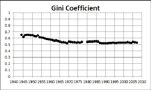
Almost thirty years after the analysis described above was done, the original author now extends it to 2005. Some of the data were obtained from an Internal Revenue Service web page and some were obtained the bound series Statistics of Income. SOI bulletin / Department of the Treasury, Internal Revenue Service, HJ4653.S7 S73. I was not able to find data for 1978 & 1979.
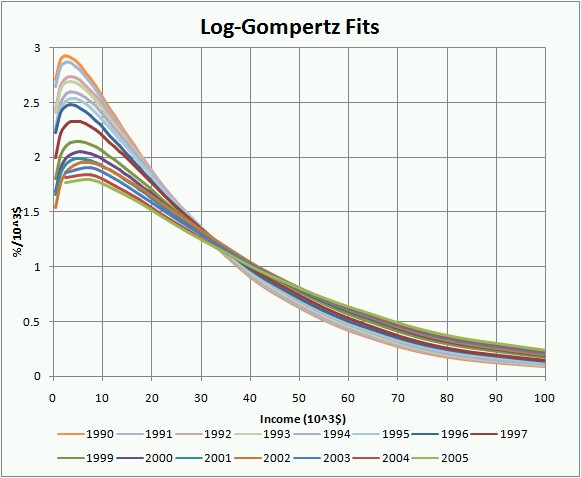
The fits to the data from 1977 to 2005 using the log-Gompertz function are shown in the following two graphs:
In the original study I fitted the log-Gompertz fits parameters (X, w) to equations for time dependence (Eq. 14). So the first thing I must do in the extension to the year 2005 is see how good the prediction is.
It is seen that the w (width) parameter energy-dependence prediction is very good, but the X (median income) is not. So I did a fit to all the data from 1945 to 2005 to the following function
 .
.
This fit is the green curve at the bottom of the graph. It will be interesting to see if the future X parameters follow this prediction.
The standard function for measuring inequality with regard to any variable x is the Gini Coefficient, the value of the Gini function:
 ,
,
for the case of the log-Gompertz distribution function. For discrete data the numerical integration is
 .
.
A value of 0 is for total equality and a value of 1 is for maximal inequality.
The result of the calculation is:
 /////
/////
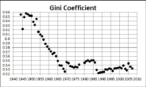
Note the close correspondence of the Gompertz width plotted above with the Gini coefficient:
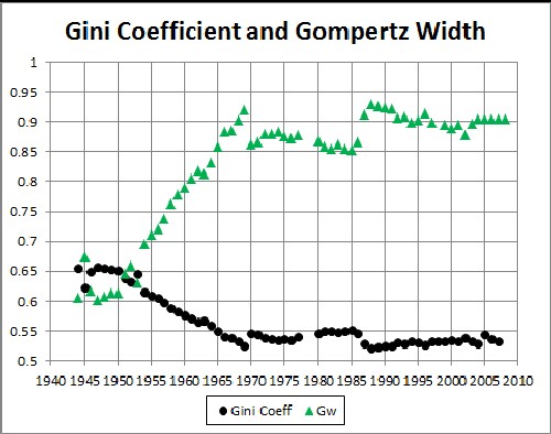
For IRS gross-income-tax data the Gini Coefficient has risen from about 0.35 to about 0.45 from 1945 to 2005. (Compare to Income Inequality in the United States.)
Another measure of income inequality is the difference between the mean (average) income and the median (mid-point) income:
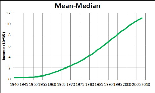
Analysis of income data for years from 2006 through 2008 is included. Notice that the difference may be headed for leveling off in future years. Mean income is heavily influenced by very high incomes.
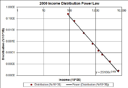
Another way to look at inequality of incomes is to fit a power law to the high tail of the income distribution:
An example of such a fit to the high tail for year-2000 data shown on a log-log plot: |
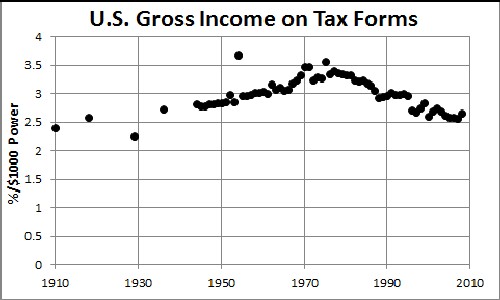
Powers of power law for U.S. gross income: |
Low powers indicate greater inequality. Note that the inequality has been on the increase since ~1970. Theory of complex webs, which economics is one, indicates that such webs are resilient to random breakdowns when the power lies between 2 and 3. However, disruption of the most highly connected nodes can easily disrupt the web.
 (Eq. 11)
  (Eq. 12)
  (Eq. 13)