
L. David Roper
http://www.roperld.com/personal/roperldavid.htm
04-Apr-2016
As the temperature of the Earth rises due to global warming one of the main consequences is that the sea level rises due to two main factors:
By studying past times when the equilibrium temperature was different than now, and thus the equilibrium sea level was different than now, one can estimate how much equilibrium sea level will rise as equilibrium temperature rises.
There is a time lag (response time) of up to a thousand years after a temperature change before the equilibrium sea level is reached. The time lag may vary depending on the environmental situation.
There is an excellent book relevant to this report The Rising Sea by Orrin H. Pilkey & Rob Young.
If the Greenland ice sheet were to all melt, sea level would rise by about 7 meters or 23 feet. If the Antarctica ice sheet were to all melt, sea level would rise by about 60 meters or 200 feet.
I use the data given in The 5 Most Important Data Sets of Climate Science and a graph for New Guinea in Florida and Bermuda Records of Sea Level to derive an equation for the change in equilibrium sea level (L in meters) as a function of the change in temperature from now (T in Celsius degrees). The temperatures (relative to 1990) to go with the sea-level data from the second reference were taken from the Vostok Antarctica ice core data with a variable factor to allow for the fact that Antarctica temperature changes are larger than average earth temperature changes; the factor searched to 0.64.
The cubic function for equilibrium-sea-level relative to now as a function of equilibrium temperature relative to now is
L = T (0.54 T2 + 0.39 T + 7.7):
The points chosen during the last Major Ice Age (125,000 ybp to 20,000 ybp) are for maxima and minima. In the interest of truthfulness, not all the other data points in the 2nd reference fit the curve so well.
The shape of the fit curve cries out for a physical explanation. Try this one for size:
The inflection point is at -0.24 C° lower than now. That is, we are living during an Earth temperature that is near the minimum of change in equilibrium sea-level rise with changing temperature:
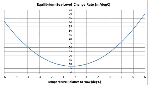
Various references (1, 2, 3, 4) give the equilibrium sea-level rise for thermal expansion of 0.7 meters per Celsius degree change in temperature. That rise is negligible relative to the equilibrium curve given in the figure above (7.6 m/deg now and 70 m/deg at 6 C° relative to now at the right edge of the curve). So most of the equilibrium rise in sea level is due to melting ice.
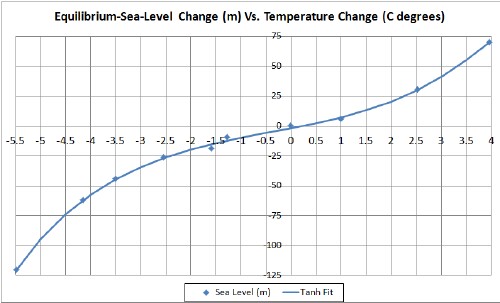
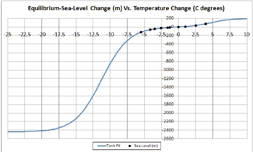
Another more physically realistic approach is to fit the sea-level-change data using two hyperbolic tangents:
The best fit is shown in the following graph:
 |
This graph shows the fit projected to the asymptotic temperature-change regions. The negative asymptote is Snowball Earth (all land covered with ice) and the positive asymptote is an ice-free Earth or at least no ice on land. Some papers indicate that the sea level was at least 160 meters below now during Snowball Earth. Although the best fit, shown above, is about 2400 meters, a reasonably good fit can be obtained with 500 meters. The following graph shows a fit with the sea level fixed at 200 meters less than now when the Snowball-Earth temperature is set at -65C° lower than now: |
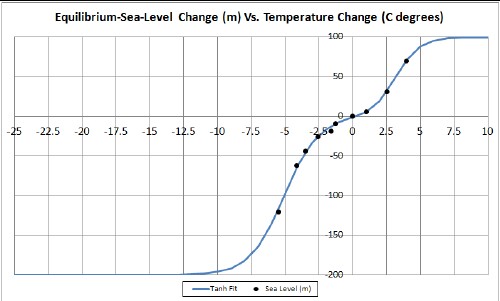 |
More data at larger temperature changes are needed to have confidence in the values of the asymptotes.
Temperatures calculated for global warming can be converted to approximate equilibrium-sea-level rises by using the equation given above. However there is a time lag of perhaps 1000 years, so immediate-sea-level rises would be much smaller. (Actually there may be different time lags for different Earth situations. Here I use only one time lag.) Since that time lag is not known, I do the following calculation for five different hyperbolic time constants: 500 years, 1000 years, 1500 years, 2000 years and 2500 years. (The time constant for the hyperbolic tangent is twice the exponential time constant for large argument of the hyperbolic tangent.)
The non-equilibrium sea-level equation with exponential time lag ![]() is
is
 .
.
The t1 is the year 2010 and n is the number of years from 2010.
Here is an example of the Excel coding:
{=SUM(($C$5:C12-$C$4:C11)*(0.54*($C$5:C12-$C$4:C11)^2+0.39*($C$5:C12-$C$4:C11)+7.7)*TANH((A12-$A$5:A12)/$E$2))} (The curly bracket surrounding the term makes it into an array; it must be entered by holding down the SHIFT & CTRL keys while pressing the ENTER key.)
In my web page Global Warming Prediction I report on a calculation of predicted Earth temperatures for several possible futures taking into account peak oil, peak natural gas and peak coal. Two of them are:
Least case: Standard parameters are used and no triggering of Earth states occurs:
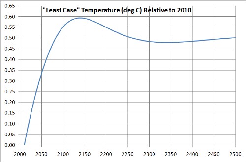
Peak fossil fuels causes the temperature peak.
Worst case: Standard parameters are allowed to change for the worse and massive carbon release from the Earth occurs:
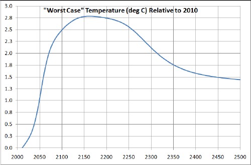
Here the temperature peak is due to both peak fossil fuels and to an assumed later peaking function for releasing carbon from the Earth.
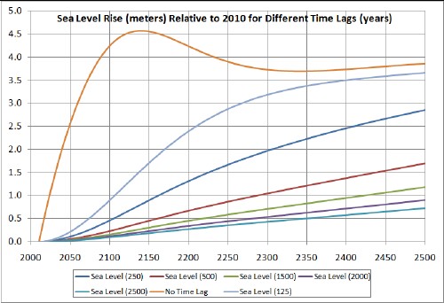
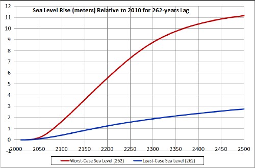
Using the non-equilibrium sea-level equation with time lag given above for five different exponential time constants and for no time lag, the non-equilibrium sea level curves for these two cases are:
Least case:
Worst case:
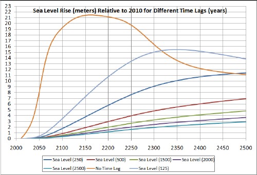
The numbers in the legend refer to the time constant in years of the exponential for large argument of the hyperbolic tangent. (The time constant for the hyperbolic tangent is twice the exponential time constant.)
After completing the above work I began to wonder if one could fit recent sea-level rises by varying the time constant in the hyperbolic tangent part of the equation. I used the recent data in the first graph of http://en.wikipedia.org/wiki/File:Recent_Sea_Level_Rise.png:
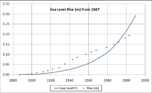
The curve is calculated from the fit of sea level vs temperature given below for a 523-years hyperbolic time constant.
The fit was essentially the same for both the least-case temperature and the worst-case temperature. The resulting fit of sea level versus temperature is:
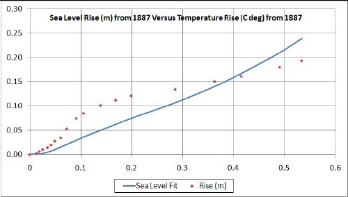
The hyperbolic time constant searched to 523 years, even when the search was started from near zero years and 10,000 years, which corresponds to an exponential time constant of 262 years.
So, it appears that the sea-level rise by 2100 will be between 0.44 and 1.7 meters.
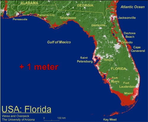
Here is what the sea level will look like in Florida when it rises 1 meter higher than now:
Adapting to sea level rise in Virginia Beach
This work was greatly benefited by several papers by Prof. Stefan Rahmstorf.
Various references (1, 2, 3, 4) give the sea-level rise for thermal expansion as follows:
The following graphs show the calculated sea-level rises for the least-case and worst-case temperature rises used above with a 10-year time constant for the top 500 meters and with a 1000-year time constant for the bottom average 3300 meters:
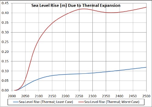
The sea-level thermal-expansion equation with exponential time lags of 10 years for the top mixed layer and 1000 years for the bottom thick layer is
 .
.
The t1 is the year 2010 and n is the number of years from 2010.
Here is an example of the Excel coding:
{=SUM(($C$5:C12-$C$4:C11)*(0.1*TANH((A12-$A$5:A12)/10)+0.6*TANH((A12-$A$5:A12)/1000)))} (The curly bracket surrounding the term makes it into an array; it must be entered by holding down the SHIFT & CTRL keys while pressing the ENTER key.)
Comparing these curves with the last graph shows that the sea-level rise due to thermal expansion is small compared to total sea-level rise.The thermal sea-level rise is between 0.06 and 0.26 meters by 2100; compare that to the total sea-level rise by 2100 of between 0.44 and 1.7 meters. The difference is a factor of about 7. If there were no time lags for both ocean layers, the sea-level rise due to thermal expansion would be between 0.4 and 1.7 meters by 2100, which would be equal to the total.
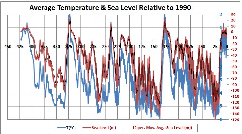
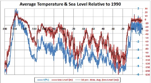
Using Earth average temperature changes from the Vostok Antarctica ice core data, that are larger than average earth temperature changes by a factor of 0.64 as determined above, and the cubic equation that relates the sea level to the temperature change, the following graphs show the calculated sea level for the last four Major Ice Ages:
 |
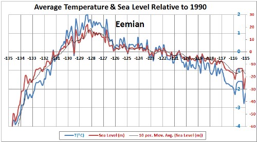
This shows the last Major Ice Age including the two Major Interglacials at each end. |
The sea-level calculation is for equilibrium. The instantaneous sea level might be somewhat lower depending on the time constant for reaching equilibrium with changing temperature. In fact, the excellent https://en.wikipedia.org/wiki/Eemian web page gives a lower sea level at Eemian peak: 4-6 meters. |
|
The black curves are 10-interval running means, to approximately allow for the fact that the cubic equation is for equilibrium sea level. (The average time interval = 131 years, the standard deviation = 159 years, the maximum = 1927 years and the minimum = 5 years; therefore, the running mean of 10 intervals averages to about 1500 years.)
This rough calculation yields sea levels between +22 meters and -149 meters compared to the 1990 level. The average = -45 meters and the standard deviation = 36 meters.
Global Ice Mass Loss
Roper Global-Heating Web Pages
L. David Roper interdisciplinary studies
L. David Roper, http://www.roperld.com/personal/roperldavid.htm; roperld@vt.edu
 This shows the last Major Interglacial (
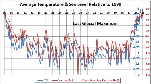 This shows the