L. David Roper
http://www.roperld.com/personal/roperldavid.htm
24 May, 2016
For the details of and the references for the equations given here see
http://www.roperld.com/science/GlobalWarmingprediction.htm .
 short tons.

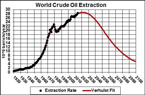
 barrels.
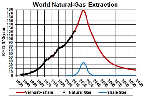
 1012 ft2.
The carbon emissions for fossil fuels are:
![]() ,
,
![]() and
and
![]() ,
,
assuming that 75% of each of the three fossil fuels is burned for fuel. Thus,
![]() .
.
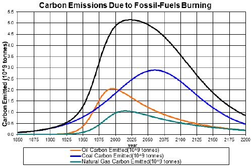
The assumption is made here that the fossil fuels are burned in the year they are extracted.

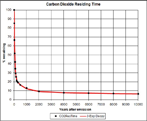
for each year tn. The factor 0.47 is the canonical factor for converting carbon emissions (109 tonnes/year) to carbon-dioxide concentration (parts per million by volume, ppmv) in the atmosphere. The three exponentials represent the carbon-dioxide residence time. Below, the possibility of this factor increasing with concentration will be considered. The three exponentials yield the following CO2-concentration decay curve:
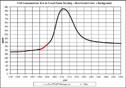
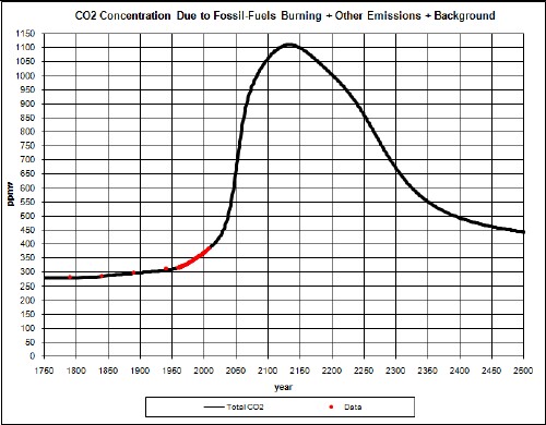
Inserting the fossil-fuels emissions in the equation yields:
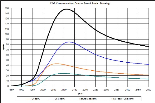
Note that the carbon-dioxide peaks are several decades later than the fossil-fuels extraction peaks shown in the graphs above, due to the carbon-dioxide residence time.
Before fossil fuels were starting to be burned for energy, there was already a background concentration of carbon dioxide in the atmosphere of about 280 ppmv. Adding that background to the carbon-dioxide concentration due to burning fossil fuels yields:
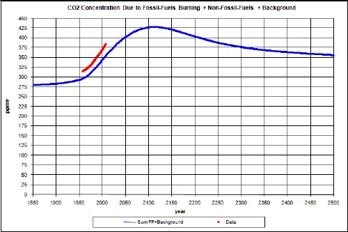
Note that the measured data are above the concentration due to fossil fuels, as it should be because there are other sources of carbon emissions, such as deforestation.
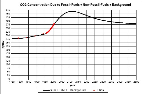
Possibly a good approximation for non-fossil-fuels (NFF) emissions is that its contribution to carbon-dioxide concentration is proportional to the fossil-fuels concentration. Rational for this approach is that the amount of deforestation, soil depletion, etc. is probably proportional to the amount of fossil fuels burned. Without fossil fuels these activities could not occur anywhere near the intensity that they do occur.
A linear fit yields a background concentration of about 292 ppmv, well above 280 ppmv, the known background concentration. It is assumed that this is due to pre-fossil-fuels emissions due to intensive agriculture and early industrialization. A hyperbolic tangent is used to represent the pre-fossil-fuels rise from c1700 to c1900:
I use a climate sensitivity of 3 degrees celsius for CO2 concentration doubling to calculate the approximate temperature change relative to year 1700, dT (in Celsius degrees), due to a change in CO2 concentration (in ppmv). The equation is:
for year tn relative to the concentration C0 for a reference year (1700 AD). The s=3 factor is the climate sensitivity that makes the climate sensitivity factor be for doubling of the CO2 concentration in the atmosphere, as it is defined. (Climate sensitivity is supposed to include the effects of fast feedback mechanisms, both positive and negative, in other variables caused by changing the CO2 concentration.)
An equivalent version of the equation is
 , where C(t0) = C0 .
Besides the climate sensitivity, one should allow for the fact that the ocean absorbs much of the solar energy impinging on the Earth and then slowly releases some of the heat energy to the atmosphere. There is a climate response function that represents the atmospheric temperature time delay after carbon is inserted into the atmosphere. The function is given by the data points in the following graph:
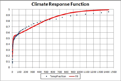
The x-axis the number of years after the carbon dioxide is inserted into the atmosphere.
The two-hyperbolic-tangent fit is good because the data errors are large. The function is
![]()
A better fit could be obtained with three hyperbolic tangents, but the errors on the data do not justify it.
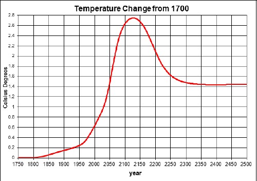
The resulting temperature change relative to 1700 due to fossil-fuels burning and non-fossil-fuels emissions is:

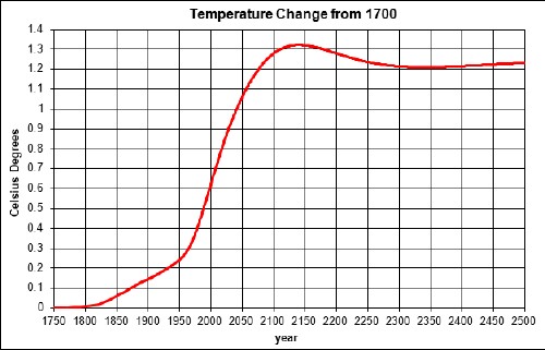
An unknown amount of global dimming should be subtracted from this curve; it is probably only a few tenths of a degree or smaller and quite variable with time.
The peak would be higher if it were not for the time delay between carbon emission and the atmospheric temperature. The asymptotic temperature is the same for both calculations, even though the ocean keeps some of the energy, because the climate sensitivity accounts for that.
Suppose that the oceans and the vegetation reach a saturation point for high carbon-dioxide concentration such that the 0.47 factor doubles to 0.94 according to a hyperbolic tangent centered at 450 ppmv with a width of 25 ppmv. Then the concentration will be
The temperature would be

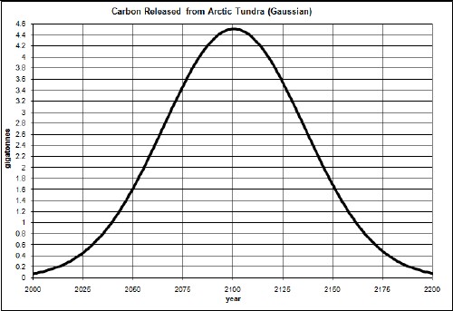
Assume that global warming causes a large amount of carbon to be released into the atmosphere in the Arctic according to
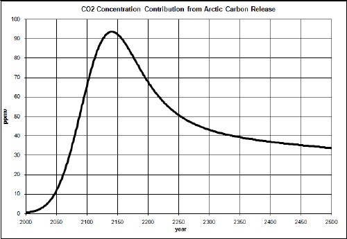
The contribution to the carbon-dioxide concentration is

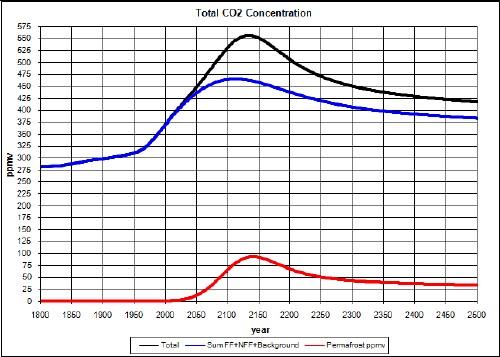
So, the total carbon-dioxide concentration is now

The temperature would be

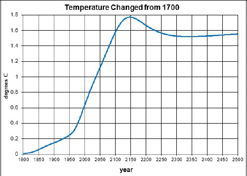
Suppose both Arctic carbon release and high carbon-dioxide concentration feedback on the concentration occurs:
The temperature would be

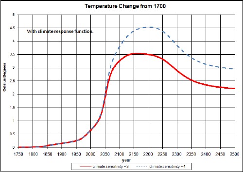
The dashed curve is for a climate sensitivity changing from 3 to 4 by a hyperbolic-tangent function:
![]()
Global Warming Web Pages of L. David Roper
Global Warming Graphs